SVM Classification
Classifies data (both linear and non-linear) by clustering it into the most distant and distinct groups possible.

Algorithm
The basic premise behind SVM Classification is following the idea of finding the maximum-margin hyperplane (MMH) in order to minimize the chances of misclassification for the training points. The SVM algorithm runs through the possible ways to divide a data set into classifications using a "hyperplane"; it then chooses the classification with the largest margin, or separation, between the classes' boundary points, called support vectors.
The following shows a simplified example of this maximal margin division process, with the defining support vector data points circled.
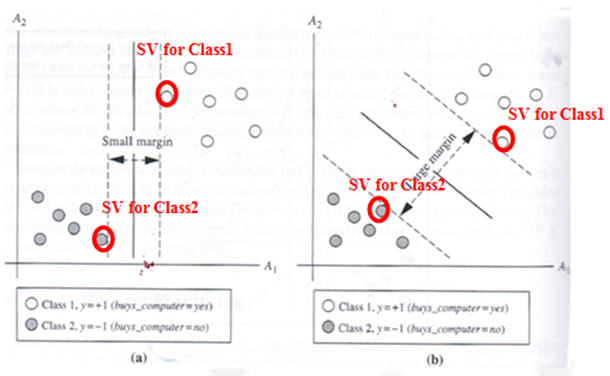
Figures (a) & (b): Support Vector Machine Algorithm Overview Diagram
In Figure (a), the data is separated by a vertical "hyperplane," resulting in a small margin between the two classes.
In Figure (b), the data is separated by a diagonal "hyperplane," resulting in a larger margin between the two classes.
The SVM Classification algorithm would choose the classification of Figure (b) over the classification of Figure (a) due to the larger margin.
The algorithm mathematically calculates the geometric distances of the data points to the boundaries (iteratively), which becomes a problem of solving well-understood mathematical quadratic equations.
The goal of the common SVM formulation is to find the optimal linear decision boundary in term of available training points. The above example shows a data set that is considered to be linearly separable. However, the following diagram shows a data set where it is not possible to draw a straight line to separate the classes. This is referred to as the data set having a "nonlinear decision boundary."
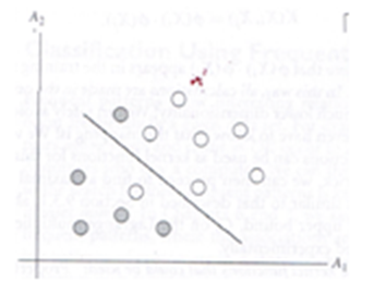
Figure ©): Example of non-linearly separable data, meaning it is not possible to draw a straight line to separate the classes.
In addition to acting as a linear model, the SVM algorithm is able to handle noisy and non-linear separable situations using the concepts of Soft Margin and Kernel Trick.
- The Soft Margin idea manipulates the original SVM optimization problem (so-called primal hard margin) to behave more flexibly for adapting to tolerable non-linearity (noise).
- Kernel Tricks are easy and efficient mathematical transformations of the data to higher dimensional space.
- The Kernel Trick is an easy and efficient mathematical way of mapping data sets into a higher dimensional space; where it finds a "hyperplane" with the hope of make the linear separable representation of the data. This is simply the method of mapping observations from a general set, S, into an inner product space, V (equipped with its natural norm), without ever having to compute the mapping explicitly.
- The three Kernel Methods currently supported by the Team Studio SVM Classification operator are the Dot Product/Linear, the Polynomial Kernel, and the Gaussian Kernel.
- Normalization Type
- Within the SVM algorithm, the Normalization type sets the mathematical approach to normalizing the SVM Classification data. The following formulas are used for normalization options:
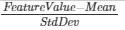
Option Description Formula Standardization Standardization normalization approach is the default approach FeatureValue Unit Vector Unit Vector normalization approach is helpful when the modeler needs the data to be in a smaller scale (that is, have smaller values). FeatureValueSampleNorm Mixed Performs both Standardization and Unit Vector normalization on the data. - None No normalization. - The SVM Classification algorithm is currently only supported for Hadoop data sources, as follows:
- For the Team Studio Hadoop (MapReduce) version, the Team Studio SVM Classification operator implements the primal form of the L2- Regularized, multi-class, cost sensitive Hinge loss function Introduced by Crammer and Singer (2001) [3] along with the idea of explicit random feature mappings for approximate the kernel trick process. The random feature mappings are established based on some classical theorems of harmonic analysis (Bochner 1994 and Schoenberg 1942).
- The supported Kernel functions for Hadoop sources are the Linear/Dot Product, Polynomial, and Gaussian functions.
- For the Gaussian function, as a shift invariant kernel, Team Studio implements the Random Fourier transformation presented by Rahimi and Recht (2007).
- For the Polynomial function, Team Studio implements the Random Maclaurin Feature Maps presented by Kar and Karnick (2012).
Configuration
The following configuration parameters are the minimum settings required to use SVM Classification.
| Parameter | Description |
|---|---|
| Notes | Any notes or helpful information about this operator's parameter settings. When you enter content in the Notes field, a yellow asterisk is displayed on the operator. |
| Dependent Column |
A dependent column must be specified for the SVM Classification. Select the data column to be considered the dependent variable for the classification. This is the quantity to model or predict. The dependent column can be either categorical or continuous.
The cardinality of the dependent column should not be greater than 1000. Therefore, there can be at most 1000 classes in the model. |
| Maximum Number of Iterations |
Controls the number of times the SVM Classification algorithm is run against the data.
Default value: 100. |
| Columns |
Sets the Independent Variable data columns to include for the decision tree training. You must specify at least one column.
Click Select Columns to open the dialog box for selecting the available columns from the input data set for analysis. For more information, see Select Column Dialog Box. |
| Kernel Type |
Specifies which implementation of a data transformation algorithm, or "kernel trick", to use to represent data in a higher dimensional space. Methods (KMs) are a class of data transformation algorithms (equations) for pattern analysis, where the goal is to find and study general types of relations (for example, clusters, rankings, principal components, correlations, and classifications) in general types of data (such as sequences, text documents, sets of points, vectors, images, etc.).
According to Mercer's Theorem (1909), the inner product of two data vectors in higher-dimensional space can be represented in linear space by a mathematical formula, or kernel representation. Specifically, it states that every semi-positive definite symmetric function is a kernel. A kernel is a primal space representation of an inner product of two data vectors in higher dimensional space: f(xi) * f(xj) Kernel type options are as follows.
The Polynomial and Gaussian kernel types should be chosen when the modeler believes the data source is not linearly separable, or has a rough Decision Boundary. When this is the case, it is recommended that the modeler try implementing the SVM Classification model with both Polynomial and Gaussian Kernel Types and comparing the results for best fit. |
| Polynomial Degree | Specifies the value of the exponent,
d, for the polynomial kernel method implementations.
For Natural Language Processing (NLP) problems, the most common degree is 2, because using larger degrees tends to leading to overfitting (http://en.wikipedia.org/wiki/Polynomial_kernel). However, for other very sparse, large data sources, such as Forest Cover use case, a good degree is 10 - many support vectors are needed to represent the non-smooth Decision Boundaries. Default value: 2. This parameter is enabled only when the Polynomial option of the Kernel Type parameter is selected. |
| Gamma (γ) | Specifies the value of the γ variable in the following Gaussian Kernel Type radial basis function:
Gamma and sometimes parameterized using
Changing the Gamma value changes the accuracy of the Gaussian model. The modeler should use trial and error with cross validation in order to assess what value is best for the given data set. This variable is typically set relative to 1 over the number of independent variables, or dimensionality, of the model. For example, if there were 50 variables, it might be set to 1/50 = 0.2. Default value: 1. This parameter is enabled only when the Gaussian option of the Kernel Type parameter is selected. |
| Lambda (λ) | Represents an optimization parameter for SVM Classification. It controls the tradeoff between model bias (significance of loss function) and the regularization portion of the minimization function (variance).
The higher the Lambda, the lower chance of over-fitting. Over-fitting is the situation where the model does a good job "learning" or converging to a low error for the training data but does not do as well for new, non-training data. If a model does well on the training data but does not perform well on the predictions, the modeler might seek to increase the Lambda value. Default value: 0.0001. |
| Normalization Type | Sets the mathematical approach to normalizing the SVM Classification data.
The options are as follows. The Standardization normalization implements the normalization equation
The Unit Vector normalization approach is helpful when the modeler needs the data to be in a smaller scale (that is, have smaller values). It implements the equation
|
| Max JVM Heap Size (MB) (-1=Automatic) | A Java Virtual Machine data storage setting for Hadoop. |
 .
.
 .
.
 .
.
Output
- Visual Output
-
Important: To learn more about the visualization available in this operator, see Explore Visual Results.
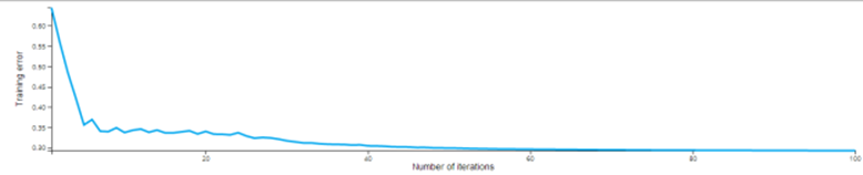
The ideal results curve would show the Training Error gradually reducing until it plateaus and flattens out at the minimal attained error rate. This shows the number of iterations at which the model has stopped getting more accurate overall.
In the above example, the Training Error seems to minimize after 60 Iterations. The modeler could rerun the model reducing Number of Iterations to 60 since going beyond that doesn't seem to improve the accuracy of the model.
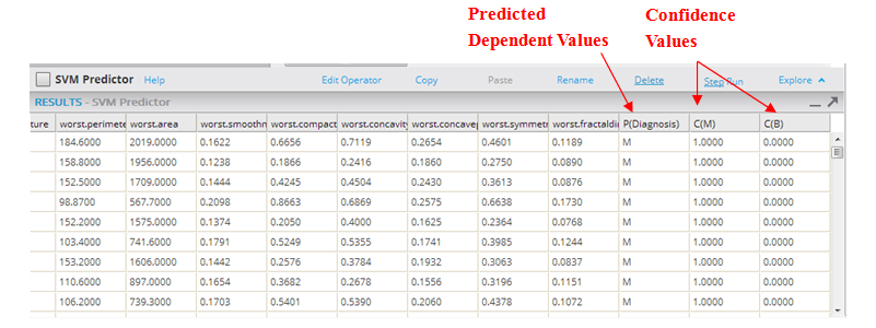
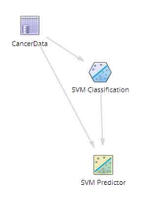
Note: If the results curve continues to oscillate, it is an indication of too much noise in the model. The modeler might try adjusting the Lambda configuration parameter or choosing a different Kernel Type option.SVM Classification models need additional operators added to them in order to analyze their effectiveness. Often, they are followed by an SVM Predictor which provides the prediction value for each data row compared against the actual data set training value and the associated confidence level. It is also common to add a ROC operator to quickly assess the quality of the model. See the Example section for an illustration.
The output from the SVM Predictor operator shows the predicted Dependent Value for each data instance, along with its associated confidence values.
- The P(Diagnosis) column uses a threshold assumption of > than 50% confidence that the prediction will happen. For example, if the confidence C(M) is over .50, the prediction value displayed is "Malignant," indicating a cancerous cell.
- The C(M) column indicates the confidence that the dependent value will be M for malignant cell. Note: usually confidence values are a decimal value that represents the % of confidence in its result.
- The C(B) column indicates the confidence that the Dependent value will be B for Benign cell.
Adding additional Scoring operators, such as a ROC graph, are also helpful in immediately assessing how predictive the Random Forest model is. For the ROC graph, any AUC value over .80 is typically considered a "good" model. A value of 0.5 just means the model is no better than a "dumb" model that can guess the right answer half the time. - Data Output
- None.