Logistic Regression (DB)
The Logistic Regression operator fits an s-curve logistic or logit function to a data set to calculate the probability of the occurrence of a specific categorical event based on the values of a set of independent variables.

Information at a Glance
For more detailed information on logistic regression, use cases, and this operator, see Probability Calculation Using Logistic Regression.
Algorithm
The database implementation for logistic regression implements a binomial logistic regression algorithm (and a StepWise Feature Selection capability to avoid over-fitting a model with too many variables). Binomial or binary logistic regression refers to the instance in which the criterion can take on only two possible outcomes (for example, "dead" vs. "alive", "success" vs. "failure", or "yes" vs. "no").
For binomial logistic regression, the Logistic Regression operator computes a probability model for the likelihood of the Value to Predict based on the values of causal independent variables.
The binomial logistic regression Algorithm uses the Iteratively Re-weighted Least Squares (IRLS) method of fitting a binomial logit function to a data set.
- The Team Studio Logistics Regression Operator applies a binomial regression by assuming the dependent variable is either the Value to Predict or Not (Value to Predict).
- For binomial logistic regression, the dependent variable must have only two distinct possible discrete values, such as "yes/no" or "0/1".
- For binomial logistic regression, the operator requires numeric independent variable values. However, if categorical independent variables (such as eye color) are specified in the source data set, the Team Studio algorithm automatically converts them into "levels" behind the scenes before running the logistic regression training.
The values of categorical variables are often referred to as levels. In Team Studio, each level is treated as a Boolean value. For example, the "eye color" variable might be represented by three Boolean levels, IsBlue?, IsGreen?, and IsBrown?.
Configuration
As of Team Studio 6.3, the Logistic Regression operator searches the parameter space of λ and α and automatically selects the highest performing model. To use this feature, provide either a comma-separated list (for example, .1,.2,.3) for λ or α, or start:end:step (for example, 0:1:.1). The operator computes all possible λ and α combinations, and the output from the operator is the model with the highest classification performance. The results of every parameter combination are visible in the results console under the Parameter optimization results tab.
| Parameter | Description |
|---|---|
| Notes | Any notes or helpful information about this operator's parameter settings. When you enter content in the Notes field, a yellow asterisk is displayed on the operator. |
| Dependent Column |
The quantity to model or predict. A dependent column must be specified for the logistic regression. Select the data column to be considered the dependent variable for the regression.
The dependent column is often a categorical type, such as eye color = blue, green, or brown. |
| Value to Predict |
Required for binomial logistic regression only. You must specify a
Value to Predict that represents the value stored in the dependent variable column that should be the event to analyze.
For example, the Value to Predict could be Active vs. Inactive. This specifies the value that the dependent variable must have to be considered a "successful" event in the logistic regression. For binomial logistic regression, the value of the Dependent Column that indicates a positive event to predict is required input. For example, the value to predict could be "Yes" for defaulting on a loan. Note: The value of this column must match the data as it is stored in the database that matches how it appears in the data explorer. If you define a Boolean dependent column with 1s and 0s, you must use 1 or 0 as the
Value to Predict. If the column uses Trues and Falses, you must use "True" or "False" as the
Value to Predict.
|
| Maximum Number of Iterations | The total number of regression iterations that are processed before the algorithm stops if the coefficients do not converge, or show relevance. This parameter must be an integer value >= 1.
Default value: 10. |
| Tolerance | Logistic regression requires an tolerance value to be specified. This is used to determine the maximum allowed error value for the IRLS calculation method. When the error is smaller than this value, the logistic regression model training stops. This parameter must be a decimal value >= 0.
Default value: 0.0001. |
| Columns |
Specifies the independent variable data columns to include for the regression analysis or model training. At least one column or one interaction variable must be specified.
Click the Columns button to open the dialog box for selecting the available columns from the input data set for analysis. For more information, see Select Columns Dialog Box . |
| Interaction Parameters |
Enables the selection of available independent variables as those data parameters thought to have combined effect on the dependent variable.
Creating interaction parameters is useful when the modeler believes the combined interaction of two independent variables is not additive. To define an interaction parameter, click the Interaction Parameters button and select the suspected interacting data columns. If you have feature A and feature B, selecting * uses both A, B, and the interaction A*B as independent features. Selecting : means that only A*B is used in the model. |
| Stepwise Feature Selection | Specifies the implementation of StepWise Regression methodology. Setting this option to
true specifies that one of the possible Stepwise Type regression methods defined below is used, and that the
CriterionType and
Check Value must be specified.
Note: Stepwise allows the system to find a subset of variables that works just as well as the larger, original variable set. A smaller model is generally considered by data scientists to be safer from the danger of overfitting a model with too many variables.
Default value: false, meaning that all the independent variables are considered at once when running the Regression analysis and included in the model. |
| Stepwise Type | Required if
Stepwise Feature Selection is set to
Yes. Specifies the different ways to determine which of the independent variables are the most predictive to include in the model.
For these Stepwise Type methods, the minimum significance value is defined by the operator's Check Value parameter specified, and the approach for determining the significance is defined by Criterion Type. |
| Criterion Type | Required if
Stepwise Feature Selection is set to
Yes. Specifies the approach to use for evaluating a variable's significance in the Regression Model.
|
| Check Value | Required if
Stepwise Feature Selection is set to
Yes. Specifies the minimal significance level value to use as feature selection criterion in
FORWARD,
BACKWARD, or
STEPWISE regression analysis.
Default value: 0.05. Alternatively, set Check Value to 10% of the resulting AIC value without a stepwise approach. |
| Group By | Specifies a column for categorizing or sub-dividing the model into multiple models based on different groupings of the data. A typical example is using Gender to create two different models based on the data for males versus females. A modeler might do this to determine if there is a significant difference in the correlation between the dependent variable and the independent variable based on whether the data is for a male or a female. |
Output
- Visual Results
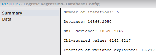
- The
Summary output displays the
Number of iterations,
Deviance,
Null deviance,
Chi-squared value, and
Fraction of variance explained statistical values.
- Number of iterations: Indicates the number of times the logistic regression re-weighting process was run. When Iteration = Maximum Number of Iterations, it flags that the regression might not have yet converged or there was a fit failure (that is, no correlation pattern was uncovered).
- Deviance: Used as a statistic for overall fit of a logistic regression model. However, this number is meaningless by itself - it should be compared against the
Null deviance value below or with its own value from previous runs of the regression.
- Deviance is the comparison of the observed values, Y, to the expected values Y predicted.
- The bigger the difference or Deviance of the observed values from the expected values, the poorer the fit of the model.
- As more independent variables are added to the model, the deviance should get smaller, indicating improvement of fit.
- Null deviance: Indicates the deviance of a "dumb" model - a random guess of yes/no without any predictor variables.
- Chi-squared value: The difference between the
Null deviance and
Deviance.
Chi-square technically represents the "negative two log likelihood" or -2LL deviance statistic for measuring the logistic regression's effectiveness.
Chi square =
Null deviance minus
Deviance.
- The hope is for the Deviance to be less than the Null deviance. Another flag for the logistic regression model not converging or there being a fit failure is having the Deviance > Null deviance, or a negative chi square. This might indicate that there is a subset of the data that is over fit on - the modeler could try removing variables and rerunning the regression.
- Fraction of variance explained: The Chi-squared value divided by the Null deviance. This ratio provides a very useful diagnostic statistic representing the percentage of the system's variation the model explains (compared to a dumb model). When analyzing logistic regression results, looking at the Chi-squared/Null deviance value provides a similar statistic to the R2 value for Linear Regressions. As a rule of thumb, any Chi-squared/Null deviance value over .8 (80%) is considered a successful logistic regression model fit.
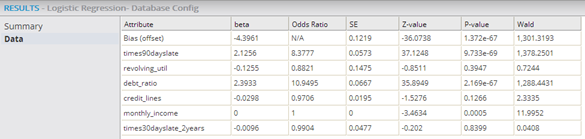
- Data Results
- The
Data output displays the statistical fit numbers for each independent variable in the model.
- Attribute: Displays the name of the independent variable.
- Dependent Value: Displays for multinomial logistic regression only. Dependent Value shows the specific categorical value for the given regression statistical data. Note that the results have a row for each Attribute/Dependent Value pair.
- Beta/Coefficient: Also represented as β, Beta is the value of the linear model Correlation Coefficient for the natural logarithms of the probability of occurrence of each independent variable in the logistic regression. Note: The Beta is also referred to as the "log scale".
- Odds Ratio: The Odds Ratio is the primary measure of the strength of a variable's impact on the results in logistic regression (that is, the "odds" of the event happening given the value of the independent variable). It represents a probability ratio of P/(1-P), where P is the probability of an event happening and 1-P is the probability of it not happening. Note that it is actually calculated by taking the β coefficients and finding exp(B) or eB, which provides useful measure the strength of the logistic regression's independent variable impact on the outcome result. For example, a β =.75 gives an Odds Ratio of e .75 = 2.72 .75 =2.12 indicating that the probability of a success is twice as likely as the independent variable's value is increased by 1 unit.
- SE/Standard Error, or SE: Represents the standard deviation of the estimated Coefficient values from the actual Coefficient values for the set of variables. It is best practice to commonly expect + or - 2 standard errors, meaning the actual value should be within two standard errors of the estimated coefficient value. Therefore, the SE value should be much smaller than the forecasted beta/Coefficient value.
- Z-value: Very similar to the T-value displayed for Linear Regressions. As the data set size increases, the T and Z distribution curves become identical. The Z-value is the value is related to the standard normal deviation of the variable distribution. It compares the beta/Coefficient size to the SE size of the Coefficient and is calculated as follows: Z =β/SE, where β is the estimated beta coefficient in the regression and SE is the standard error value for the Coefficient. The SE value and Z-value are intermediary calculations used to derive the following, more interesting P-value, so they are not necessarily interesting in and of themselves.
- P-value: Calculated based on the
Z-value distribution curve. It represents the level of confidence in the associated independent variable being relevant to the model, and it is the primary value used for quick assessment of a variable's significance in a logistic regression model. Specifically, it is the probability of still observing the dependent variable's value if the
Coefficient value for the independent variable is zero (that is, if
P-value is high, the associated variable is not considered relevant as a correlated, independent variable in the model).
- A low P-value is evidence that the estimated Coefficient is not due to measurement error or coincidence, and therefore, is more likely a significant result. Thus, a low P-value gives the modeler confidence in the significance of the variable in the model.
- Standard practice is to not trust Coefficients with P-values greater than 0.05 (5%). Note: a P-value of less than 0.05 is often conceptualized as there being over 95% certainty that the Coefficient is relevant. In actuality, this P-value is derived from the distribution curve of the Z-statistic - it is the area under the curve outside of + or - 2 standard errors from the estimated Coefficient value.
- Note: The smaller the P-value, the more meaningful the coefficient or the more certainty over the significance of the independent variable in the logistic regression model.
- Wald Statistic: Used to assess the significance of the Correlation Coefficients. It is the ratio of the square of the regression coefficient to the square of the standard error of the coefficient as follows. The Wald Statistic tends to be biased when the data is sparse. It is analogous to the t-test in Linear Regression.
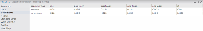
Note: When assessing the Data tab of the Logistic Regression operator, a modeler mostly cares about the odds ratios, which indicate strength of the correlation between the dependent and independent variables, and the P-values, which indicate how much not to trust the estimated coefficient measurements. - Coefficient Results (multinomial logistic regression)
- For multinomial logistic regression results, the Correlation Coefficient value for each of the specific dependent variable's categorical values is displayed.
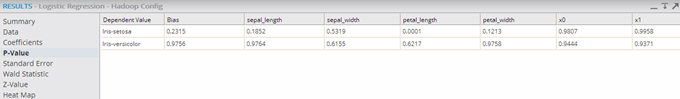
- P-Value Results (multinomial logistic regression)
- For multinomial logistic regression results, the P-Value for each of the specific dependent variable's categorical values is displayed.
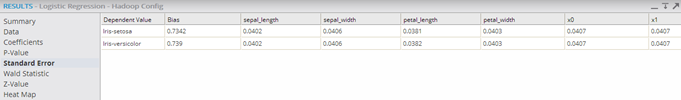
- Standard Error Results (multinomial logistic regression)
- For multinomial logistic regression results, the SE value for each of the specific dependent variable's categorical values is displayed.
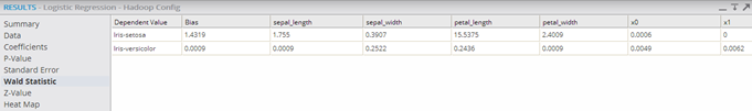
- Wald Statistic Results (multinomial logistic regression)
- For multinomial logistic regression results, the Wald Statistic for each of the specific dependent variable's categorical values is displayed.
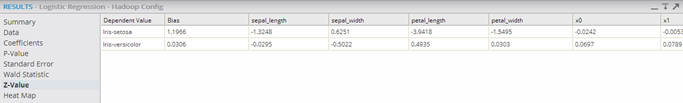
- Z-Value Results (multinomial logistic regression)
- For multinomial logistic regression results, the Z-Value for each of the specific dependent variable's categorical values is displayed.
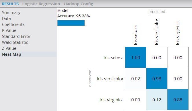
- Heat Map Results (multinomial logistic regression):
-
For multinomial logistic regression results, the Heat Map displays information about actual vs. predicted counts of a classification model and helps assess the model's accuracy for each of the possible class values.
In the following example, the Heat Map shows an overall model accuracy of 95.33% with the highest prediction accuracy being for the class value "Iris-setosa" (100% accurate predictions) versus the lowest being for the "Iris-virginica" (88% accurate predictions).
To learn more about the visualization available in this operator, see Exploring Visual Results.
- Data Output
- A file with structure similar to the visual output structure is available.