Linear Regression - MADlib
Team Studio supports the MADlib open source implementation of the Linear Regression algorithm.

Algorithm
The MADlib Linear Regression operator applies an Ordinary Least-Squares (OLS) linear regression algorithm to the input dataset. It is processed using the least squares method of regression analysis, meaning that the model is fit such that the sum-of-squares of differences of observed and predicted values is minimized.
More information including general principles can be found in the official MADlib documentation.
Configuration
| Parameter | Description |
|---|---|
| Notes | Any notes or helpful information about this operator's parameter settings. When you enter content in the Notes field, a yellow asterisk is displayed on the operator. |
| MADlib Schema Name | Schema where MADlib is installed in the database. MADlib must be installed in the same database as the input dataset. If a "madlib" schema exists in the database, this parameter defaults to madlib. |
| Model Output Schema Name | The name of the schema where the output is stored. |
| Model Output Table Name | The name of the table that is created to store the Regression model. Specifically, the model output table stores:
[ group_col_1 | group_col_2 | ... |] coef | r2 | std_err | t_stats | p_values | condition_no [| bp_stats | bp_p_value] See the official MADlib linear regression documentation for more information. |
| Drop If Exists | |
| Dependent Variable | Required. The quantity to model or predict. |
| Independent Variables | Click
Select Columns to select the available columns from the input data set for analysis.
Select the independent variable data columns for the regression analysis or model training. You must select at least one column. |
| Grouping Columns | You can set at least one column to group the input data and build separate regression models for each group.
Click Select Columns to open the dialog box for selecting the available columns from the input dataset for grouping. |
| Heteroskedacity Stat | Set to true (the default) to output two additional columns to the model table. |
| Draw Residual Plot | Set to
true (the default) to output Q-Q Plot and Residual Plot graphs for the linear regression results.
|
Output
When assessing the Data tab results of the Linear Regression Operator, a modeler focuses mostly the Coefficient values, which indicate the strength of the effect of the independent variables on the dependent variable, and the associated P-values, which indicate how much not to trust the estimated correlation measurement.
- Visual Output
- The MADlib Linear Regression Operator results output is displayed across the
Summary and
Data sections.
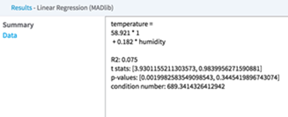
- Summary
-
The derived linear regression model is a mathematical equation linking the Dependent Variable (Y) to the Independent Variables (X1, X2, etc.). It includes the scaling or Coefficient values (β1, β2, etc.) associated with each independent variable in the model. Note: The resulting linear equation is expressed in the form of Y= β0 + β1*X1 + β2*X2 + …
The following overall model statistical fit numbers:
- R2: R2 is called the multiple correlation coefficient of the model, or the Coefficient of Multiple Determination. It represents the fraction of the total Dependent Variable (Y) variance explained by the regression analysis, with 0 meaning 0% explanation of Y variance and 1 meaning 100% accurate fit or prediction capability.
- S: represents the standard error per model (often also denoted by SE). It is a measure of the average amount that the regression model equation over- or under-predicts.
For example, if a linear regression model predicts the quality of the wine on a scale between 1 and 10 and the SE is .6 per model prediction, then a prediction of Quality=8 means the true value is 90% likely to be within 2*.6 of the predicted 8 value (that is, the real Quality value is likely between 6.8 and 9.2).
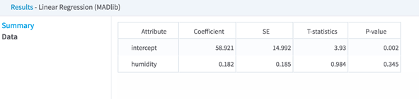
- Data
- Displays the model coefficients and statistical fit numbers for each Independent variable in the model.
- Data Output
- None. This is a terminal operator.