Example 6: Tabulating Multiple Responses and Dichotomies
The general idea of multiple response variables and multiple dichotomies is described in Multiple Responses/Dichotomies - Introductory Overview. If you are entirely unfamiliar with such variables, it is recommended that you review that section before continuing with this example. This example illustrates how the need to use such variables often arises in survey research and how they can be analyzed with the Basic Statistics and Tables module of Statistica.
An example data file with the results of a fictitious survey is included in the /Examples/Datasets directory of Statistica to demonstrate the three types of variables that can be tabulated:
Simple categorical variables,
Multiple response variables, and
Multiple dichotomies.
Simple frequency tables will first be computed in order to show how these three types of variables can be summarized; then cross-tabulation tables involving these variables will be examined.
Gender (simple categorical variable). The respondent's gender was recorded and entered as a categorical variable (Gender) into the data file (i.e., Male, Female).
Favorite fast-food (multiple response variable). The questionnaire that was used for this study asked the respondents to select their favorite (up to) three choices of commonly available fast foods from a list of 8 different types. The 8 different types of fast food that were presented to the respondents were:
(1) Hamburger
(2) Sandwiches
(3) Chicken
(4) Pizza
(5) Mexican fast-food
(6) Chinese fast-food
(7) Seafood
(8) Other ethnic or regionally popular fast-food
The three choices that each respondent made were entered into the data file as a multiple response variable, that is, their first choice was entered into variable Food_1 (first preference or favorite fast food), their second choice (if available) was entered into variable Food_2, and their third choice into variable Food_3.
Multiple identical responses were not allowed, e.g., if a respondent identified three favorite fast foods as Hamburger, Hamburger, and Hamburger, then Hamburger was only entered once as that respondent's favorite food (in variable Food_1), and the respective cells for variables Food_2 and Food_3 were left blank.
In the analysis, you could treat variable Food_1 as a simple categorical variable, and ask the question: What is the number (proportion) of respondents that mentioned the respective type of fast-food as their favorite? However, you would also be interested in how many respondents mentioned a particular type of fast food as any one of their three favorite fast foods. This question requires that you treat variables Food_1 through Food_3 as a multiple response variable; for example, if you want to count the number of respondents who chose Hamburgers as either their first, second, or third preference. This will be clarified further when the frequency table for this variable is discussed.
Favorite car (multiple response variable). Here, each subject was asked to write down the three most desirable cars (make and model) that they would like to own (if money were no object). These responses (specific brands and models) were coded into four categories:
(1) Domestic sports car
(2) Domestic sedan
(3) Foreign sports car
(4) Foreign sedan
This variable, just as the favorite fast-food variable (see above), was entered as a multiple response variable, that is, the respondents' preferences were entered into variables Car_1 through Car_3. Note, however, that in this case, the subjects could repeat the same answer three times (e.g., they could mention 3 sports cars as their three most desirable cars). In the fast-food case above, multiple identical responses were not allowed (i.e., ignored).
Recent patronage of specific hamburger restaurants (multiple dichotomy). Finally, the subjects were asked to indicate which of four different (specific) local fast-food hamburger restaurants they had visited in the two weeks prior to the survey. In this case, the data was entered such that a variable was included in the file for each specific restaurant. The four variables, Burger_1 through Burger_4, represented the following four different local restaurants:
(1) Burger Meister
(2) Bill's Best Burgers
(3) Hamburger Heaven
(4) Bigger Burger
If a respondent reported to have eaten at one or more of these restaurants recently, a 1 was entered into the respective column; if not, then it was left blank. Thus, this is a multiple dichotomy, and it is desired to tabulate the number (or proportion) of respondents that report to have eaten at each of the four restaurants in the study.
Data file. Open the example data file Fastfood.sta.
Ribbon bar. Select the Home tab. In the File group, click the Open arrow and on the menu, select Open Examples. The Open a Statistica Data File dialog box is displayed. Fastfood.sta is located in the Datasets folder.
Classic menus. On the File menu, select Open Examples to display the Open a Statistica Data File dialog box; Fastfood.sta is located in the Datasets folder.
To illustrate how each subject's responses were entered into this data file, look at the first subject (case) in the spreadsheet. The first subject was a woman, so the value Female was entered in the variable Gender. As her most favorite fast food, she chose Pizza (entered into variable Food_1), as her second favorite fast food she chose Seafood (entered into variable Food_2), and she chose no other type of fast food, so the value for variable Food_3 was left blank (i.e., missing data).
The three cars that she mentioned were coded as (1) domestic sedan, (2) domestic sports car, and (3) again as domestic sports car in the variables Car_1, Car_2, and Car_3, respectively. Finally, she responded that she ate at Burger_1 (Burger Meister) and Burger_3 (Hamburger Heaven) within the last two weeks, so values of Yes were entered for those respective variables and the values for the other two Burger variables were blank.
Overall, there were 200 respondents in the study.
Specifying the Simple Categorical and Multiple Response Variables. Now, begin the analysis by computing simple frequency tables for the simple categorical variable Gender and the multiple response variables in the study. Because some respondents have missing data for all variables Burger_1 through Burger_4 (i.e., they have not eaten in any of the four restaurants during the previous two weeks), that table will be specified separately later. By default, the cases with all missing data in the Burger variables will be excluded from the analysis, and frequency counts will be obtained only for those subjects who have eaten in at least one of the four restaurants. Alternatively, you could also select the Include missing data as an additional category for each factor check box (on the Options tab of the Multiple Response Tables dialog box).
Start the Basic Statistics module.
Ribbon bar. Select the Statistics tab. In the Base group, click Basic Statistics to display the Basic Statistics and Tables Startup Panel.
Classic menus. On the Statistics menu, select Basic Statistics/Tables to display the Basic Statistics and Tables Startup Panel.
Double-click Multiple response tables.
In the Multiple Response Tables dialog box, you can specify all three types of categorical variables, that is, simple categorical variables (such as Gender in this example), multiple response variables (such as Food_1 through Food_3 or Car_1 through Car_3), and multiple dichotomies (such as Burger_1 through Burger 4).
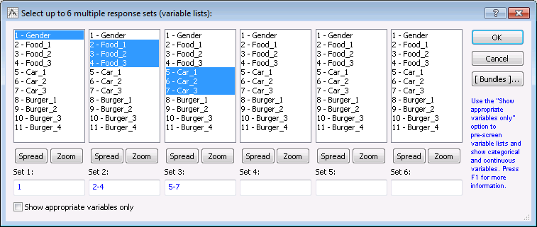
Click the Specify table (select variables) button on the Quick tab to specify the variables as shown in the following image:
As you can see, up to 6 multiple factors (simple categorical variables, multiple responses, or dichotomies) can be specified for a single table. In the first column only variable Gender is selected; STATISTICA will automatically interpret single variables (multiple response sets with only one variable) as simple categorical variables. In the second-column, variables Food_1 through Food_3 are selected, and in the third-column, variables Car_1 through Car_3 are selected. In this preliminary analysis, the simple frequency tables for all factors will be reviewed (as mentioned above, the frequency table for the multiple dichotomy factors Burger_1 through Burger_4 will be examined later).
Now click the OK button to finalize these selections and display them in the Multiple Response Tables dialog box.
Naming conventions. In the left column in this dialog box, you will see the default names for the factors in the analysis. The term factor is used here because a multiple response variable, such as food preference in this example, consists of several variables (in the data file). Note that by default the name (both short and long) for each factor will be taken from the first variable in the respective list. Also, the text labels will be taken from that variable.
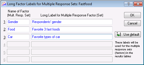
To change the names of the factors, select the Options tab, and select the User defined factor labels option button. The Long Factor Labels for Multiple Response Sets dialog box is displayed, where you can enter the desired short and long names that will be used to identify the factors in subsequent tables.
For this example, change the names of the multiple response factors slightly, so that they will more accurately reflect their meaning: Food: Favorite 3 fast foods, and Car: Favorite types of car.
Click the OK button.
Defining factors. The option buttons next to each factor (in the Multiple Response Tables dialog box, on the Quick tab) identify its type. For the first variable (Gender), the Multiple dichotomy option button is not available since that variable is a simple categorical variable. For the second and third factors, select the Multiple response option buttons.
Clear the Read all text labels check box in order to enable the Codes buttons. You can now select the codes that were used in the file to identify the different categories for the respective factor, that is, the codes that were used to identify Male and Female respondents (variable Gender), the different fast-foods in variables Food_1 through Food_3, and the different types of cars in Car_1 through Car_3.
If you do not explicitly define those codes, they will automatically be taken from the first variable in each set (factor), that is, Statistica will identify all codes in the respective variable. This will usually identify all codes that were used in that factor, but occasionally, it may happen that a particular code is not used in the first variable of a set, but only in the second or third. In that case, simply accepting the default will not identify that code. Thus, it is always advisable to enter all codes (categories) that you want to use in the tables explicitly.
To enter the codes for All factors, click any of the Codes buttons to display the Select codes for multiple response sets (factors) dialog box. Click the All button adjacent to each factor.
Then, click the OK button to close the dialog box.
Other options. Before proceeding, look at some of the other options in the Multiple Response Tables dialog box. The Paired crosstabulation check box on the Quick tab will cause Statistica to "match up" multiple response factors with equal numbers of levels, and treat them as paired variables. Paired crosstabulation is described in greater detail in the Overview.
The check boxes on the Options tab control the manner in which missing data values (i.e., blank cells in the data file) are processed. For example, by default when processing a multiple dichotomy factor, Statistica will count the number of responses equal to the Count value, and ignore all others. Alternatively, you can also treat missing data (no response at all) different from a valid data point that is not equal to the Count value. Specifically, missing data can be excluded listwise (select the Exclude missing data listwise within each multiple dichotomy set check box), that is, all cases (respondents) are excluded from the analysis if they show missing data in any of the variables included in the multiple dichotomy set. The second check box (Exclude missing data listwise within each multiple response set) works analogously, that is, it will cause cases to be excluded listwise from the analysis if they have missing data for any of the variables in the multiple response set. The last check box (Include missing data as an additional category for each factor) determines whether a separate category for missing data will be included in the frequency and cross-tabulation tables. When this check box is selected, the tabulation routines will treat (count) missing data as just another category of the respective factors.
Finally, on the Quick tab next to the Count value edit field is the Count unique responses only (ignore multiple identical responses) check box.
This check box pertains to the manner in which multiple identical responses are treated in multiple response variables. In this example, the Car factor is made up of three variables with codes that identify the types of automobile that the respondents identified as their most desirable three cars to own. Thus, it is possible that a subject selected three foreign sports cars as his or her favorite three cars, which would then result in identical codes (For_Sprt) in each of the three variables Car_1 through Car_3. The setting of this check box determines whether such multiple identical responses will be counted or ignored, that is, whether a subject naming three foreign sports cars will be counted three times (if the Count unique responses only... check box is cleared) or only once (if it is selected).
In this example, it is not of interest whether all three of a subjects' most favorite cars are of a specific type (thereby inflating the numbers by such multiple identical responses); therefore, it makes the most sense to select this check box (that is to accept the default) in order to determine the number of respondents who, for example, name a domestic sedan as one of their favorite three cars. Note that the variables making up the Food factor only contain mutually exclusive categories, since the respondents were explicitly not allowed to identify the same item as their favorite three fast-foods. Instead, the subjects had to choose from among eight fast-foods, without repeating a choice. Therefore, for factor Food, it does not matter whether this check box is selected.
Reviewing Frequency Tables for Multiple Response Factors. Click the OK button in the Multiple Response Tables dialog box to proceed with the analysis and display the Multiple Response Table Results dialog box.
For now, only the simple tabulation of frequency tables will be reviewed (the crosstabulation tables that can be produced from this dialog box will be reviewed later).
On the Options tab of the Results dialog box, select the Highlight counts > check box, and enter 100 in the corresponding edit field (so that all frequency counts greater than 100 will be highlighted in the spreadsheet). Then, on the Quick or Advanced tab, click the Frequency tables button. The interpretation of the frequency table for Gender is straightforward; the frequency tables for the other two variables are shown in the spreadsheets below.
First, look at the frequency table for the factor Food.
Overall, there were 200 respondents in the study (N=200 is shown in the upper-left corner of the spreadsheet). The Count column of the spreadsheet shows the number of respondents who mentioned the respective type of food as one of their favorite three types of fast food. Remember that only unique responses were counted and, thus, each respondent can only be counted once in this column. Therefore, you can conclude that Pizza was the most popular fast-food, mentioned either as the first, second, or third favorite by 138 respondents, Hamburger was the second most popular choice (114). All other categories of fast-food were mention by only about 40 to 50 of the respondents.
The second column of the spreadsheet expresses the raw counts relative to the number of total responses, that is, the total of the first column. So you can say that of all fast-food preferences volunteered by the respondents (remember that some only mentioned one or two), 26.44% (100*138/522) of the expressed preferences identified Pizza. In a sense, this column treats as the unit of analysis each fast-food preference mentioned by the respondents (and not the respondents themselves). By contrast, the third column of the spreadsheet shows the percentage of respondents who mentioned the respective fast-foods as either their first, second, or third preference. Here you can see that Pizza was identified as a favorite food by 69% (100*138/200) of all respondents.
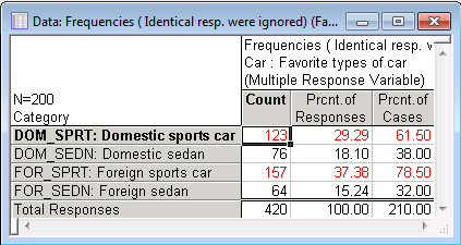
Now, look at the frequency table for the factor Car.
The interpretation of the frequency table for the Car factor is analogous. Foreign sports cars were mentioned by 157 respondents as one of their first three choices (again, remember that only unique responses are counted, thus, each respondent can only be counted once in each category); Domestic sports cars were mentioned by 123 respondents. The second column shows a 37.38% response for Foreign sports cars; this number is not readily interpretable in this case since only unique responses were counted. Thus, if a respondent identified three Foreign sports cars as his or her favorite cars, then he or she would only be counted once in this table. The numbers in the third column (Percent of cases) are more informative; for example, 78.5% of all respondents identified a Foreign sports car as one of the three most desirable cars to own.
Specifying a Multiple Dichotomy Factor. Now, return to the Multiple Response Tables dialog box (click the Cancel button in the Results dialog box) to specify the multiple dichotomy variable in this survey (patronage of particular restaurants).
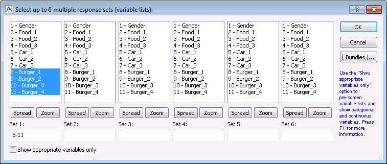
Click the Specify table (select variables) button. Clear the previously selected variables, and select Burger_1 through Burger_4 as the variables for the first set.
Click OK in the variable selection dialog box.
Next, select the Multiple dichotomy option button next to the first factor in the Multiple Response Tables dialog box. As before, you can use the User defined factor labels option button on the Options tab to enter a more appropriate name for this factor. For example, you can call this factor Patron: Recently patronized restaurants.
You still need to specify the code that was used in the multiple dichotomy factor Patron to identify whether a respondent had eaten at the respective restaurant during the two weeks prior to the survey. Specify this code in the Count value edit box below the listing of the factors. Since code number 1 (the numeric equivalent to the value Yes) was used to identify which restaurant had been visited by the respective respondent, you can simply accept the default code given in this edit box.
Remember that the way in which a multiple dichotomy variable (factor) is interpreted by Statistica is that it will treat the different variables in the set as levels (categories) of the respective multiple dichotomy factor, and then count the number of entries in those variables (categories) that are equal to the code number. All values that are not equal to the code number will be treated the same, that is, they will be ignored. Thus, you can use more "sophisticated" coding schemes for multiple dichotomies than the simple 1-0 (or nothing, i.e., missing) coding used in this example.
For example, you could have used a separate code (other than 1) to indicate that the respondent reported to have "never even considered eating there." You could enter code 2 in variables Burger_1 through Burger_4 to identify such strong negative responses toward the respective restaurants, and by specifying that code in the Count value edit field, you could tabulate those responses as well. Thus, by using different code values, a multiple dichotomy can be used to identify multiple mutually exclusive responses.
Missing data. There are some respondents who have not eaten in any of the four hamburger restaurants during the two weeks prior to the survey; in the data spreadsheet, those cases show blanks (missing values) for all four variables Burger_1 through Burger_4. By default, those cases will be excluded from the tabulation.
Alternatively, you could Include missing data as an additional category for each factor (select that check box on the Options tab). In that case, the resulting frequency table would show an additional fifth category labeled Missing, reporting the number of respondents who did not visit any of the four restaurants.
In this example, it is desired to tabulate only those respondents who visited at least one hamburger restaurant in order to see how this "market segment of hamburger-eaters" is divided among the restaurants (see below). Click the OK button to proceed to the Multiple Response Table Results dialog box.
Reviewing the Frequency Table for a Multiple Dichotomy. In the Results dialog box, click the Frequency tables button. The interpretation of the numbers reported in this table is analogous to that for multiple response variables.
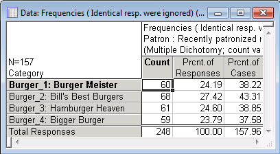
Overall, 157 respondents had eaten in one of the four restaurants in this survey (N=157); 60 respondents had eaten at Burger Meister, 68 had eaten at Bill's Best Burgers, and so on. The values in the second column (Percent of responses) express these counts relative to the total number of times that any one of the four restaurants was mentioned.
Assume that the four (fictitious) restaurants have pretty much cornered the hamburger fast-food marked in the survey city, and that the 157 respondents (out of the 200) more or less represent the total market of young adults who eat at fast-food hamburger places. In that case the values in the second column represent the market shares for the four restaurants.
For example, of all the hamburger places patronized by the respondents in the two weeks prior to the survey, Burger Meister was frequented in 24.19% of the cases, Bill's Best Burger in 27.42% of the cases, and so on. The third column (Percent of cases) reports the percent of respondents who had eaten in the past two weeks at the respective restaurants.
Remember that these percentages are expressed relative to the N of 157, that is, relative to the number of respondents who had eaten in at least one of the four restaurants. Therefore you can, for example, say that 38.22% of those respondents who had eaten in any one of the four hamburger restaurants ate at Burger Meister, 43.31% ate at Bill's Best Burger, etc.
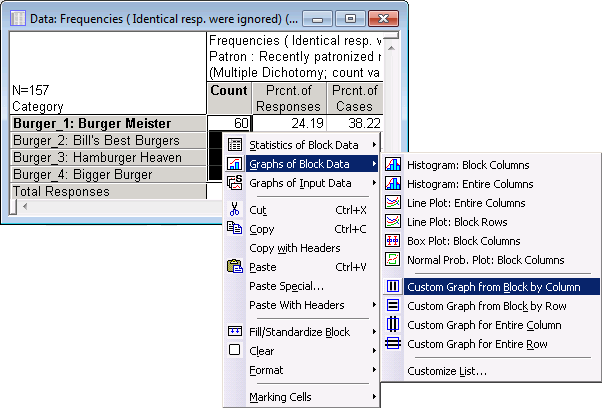
The Select graph dialog box is displayed.
In the Select Graph Category box, select 2D Graphs.
In the Select Graph Type box, select Bar/Column Plots.
In the Select Graph SubType box, select Vertical. Then, click the OK button to display the graph.
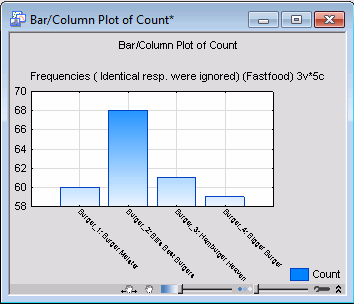
You can then further edit the resulting plot to produce a histogram summarizing these results. First, double-click the background of the graph to display the Graph Options dialog box.
Then, on the Axis: Scaling tab, specify Y left in the Axis drop-down box, change the Mode to Manual and specify 58 in the Minimum field and 70 in the Maximum field.
In the Axis: Scale Values tab, specify X in the Axis drop-down box, and under Options, change the Layout to Perpendicular. Click OK.
Crosstabulating Multiple Responses and Dichotomies. Now we'll look at some crosstabulation tables involving multiple response variables and multiple dichotomies.
Click the Cancel button in the Multiple Response Table Results dialog box to return to the Multiple Response Tables dialog box. First, let's look at the crosstabulation table of Gender by Car, that is, examine the interest in different types of cars expressed by Males and Females.
Click the Specify table (select variables) button. In the variable selection dialog box, select Gender as the only variable for Set 1, and variables Car_1 through Car_3 as the variables for Set 2. Click OK.
Next, specify the codes that were used for the Cars factor to identify the four different types of automobiles. Also, you may want to change the description of the Car factor, that is, the short and long factor labels that by default are taken from the first variable in the multiple response set (Car_1), via the User defined factor labels option button on the Options tab.
For this table, clear the Count unique responses only (ignore multiple identical responses) check box on the Quick tab. Remember that the purpose of the box is to exclude multiple identical responses from the crosstabulation table. In this instance, however, you may want to include those responses. The resulting crosstabulation table will show the total number of different types of cars identified as either the first, second, or third most desirable car, broken down by the categorical variable Gender. Now click the OK button to proceed to the Multiple Response Table Results dialog box.
For now, do not select any of the Percent check boxes on the Options tab, but simply click the Detailed two-way tables button on the Quick tab to produce the following spreadsheet.
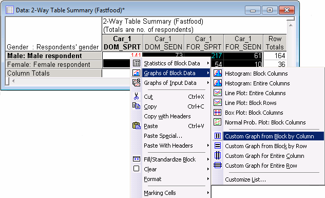
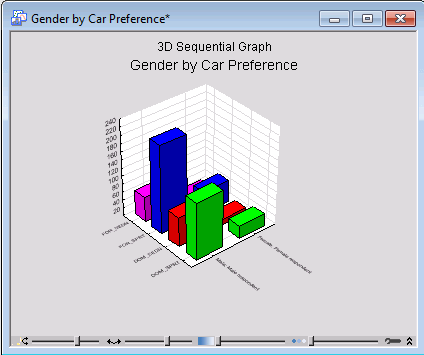
Again, it is easy to turn this spreadsheet into a graph, for example, a 3D histogram. To do this, select the first four columns and first two rows of the spreadsheet. Then right-click on your selection and select Graphs of Block Data - Custom Graph from Block by Column from the resulting shortcut menu.
The Select Graph dialog box is displayed.
In the Select Graph Category box, select 3D Sequential Graphs.
In the Select Graph Type box, select Raw Data Plots.
Finally, in the Select Graph SubType box, select Columns. Now click the OK button to produce the plot.
Looking at the above spreadsheet, it is apparent that both males and females mentioned foreign and domestic sports cars more often than sedans. The difference in the total number of cars mentioned by males and females can be attributed to the greatly different number of male and female respondents in the sample (if you look at the frequency table for Gender you will see that there were only 36 females).
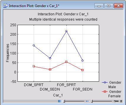
Instead of the 3D histogram, the frequencies in this table can also be expressed in a line plot. Return to the Results dialog box and click the Interaction plots of frequencies button on the Quick tab.
Here, it appears that differential preference for sports cars is more pronounced among males than among females (i.e., the line for males appears more jagged).
Relative Frequencies: Percentage of Responses vs. Respondents. Since each subject gave three responses, it is desired to first look at the percentages expressed in terms of the number of responses (total, row, and column).
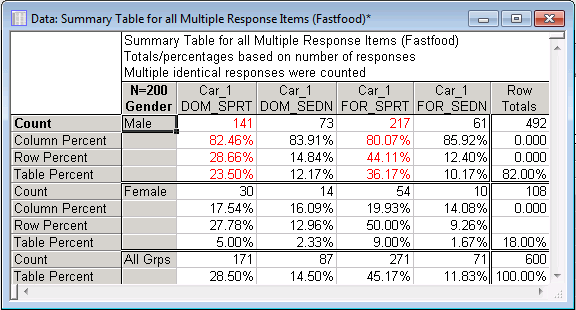
Therefore, on the Options tab, select the Number of responses option button, and then select all of the Percentage check boxes. Click the Summary button to produce the following results spreadsheet.
Each respondent named three cars; thus, the total number of responses is 600. The table percentages express the frequencies relative to that total.
For example, 141 Domestic sports cars were named by Males, which is equivalent to 23.5% (100*141/600) of all responses. The Row percentages pertain to the relative frequency with regard to all responses in the respective row. So for example, the 141 Domestic sports cars mentioned by Males represents 28.66% (100*141/492) of all cars named by Males. Accordingly, the Column percentages represent the relative frequencies with regard to the total number of responses in that column: Of all Domestic sports cars that were named, 82.46% (100*141/171) were named by Males.
Because the Count unique responses only (ignore multiple identical responses) check box on the Multiple Response Tables dialog box - Quick tab was cleared, it makes little sense to express the percentages in terms of the number of respondents. Remember that in the two-way table shown above some subjects are counted more than once in a single cell (if they, for example, mentioned more than one Foreign sports car).
If you select the Count unique responses only (ignore multiple identical responses) check box on the Multiple Response Tables dialog box - Quick tab, and then on the Multiple Response Table Results dialog box - Options tab, select the Number of respondents option button, the summary table would look like this:
The interpretation of the percentages in this table is now different from the previous spreadsheet. For example, 100 Males mentioned a Domestic sports car as either their first, second, or third choice for a car they would like to own. The respondents counted in that cell represent 50% (100*100/200) of all respondents; they represent 81.3% (100*100/123) of all respondents (Male and Female) who mentioned a Domestic sports car as either their first, second, or third choice, and they represent 60.98% (100*100/164) of all Male subjects.
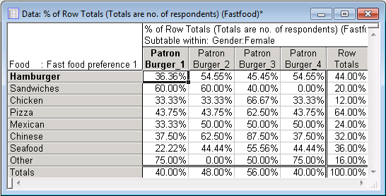
Reviewing a Three-Way Table. Finally, you can determine whether there are preferences for different hamburger restaurants among male and female respondents if they mention a particular type of favorite food. In other words, crosstabulate Gender by Food by Patron.
Return to the Multiple Response Tables dialog box and specify those three factors as before, that is, Gender as a simple (single) categorical variable, Food as a Multiple response variable, and Patron as a Multiple dichotomy.
Click the OK button in this dialog box. In the Multiple Response Table Results dialog box, on the Options tab, select the Percentages of row count check box and the Number of respondents option button. On the Advanced tab, select the Display selected %'s in sep. tables check box.
These choices will enable you to review the three-way table, one two-way table at a time, first for Males and then for Females. Moreover, the percentage tables (of row counts of numbers of respondents) will be displayed in separate tables. Click the Detailed two-way tables button on the Advanced tab to display the percentage tables.
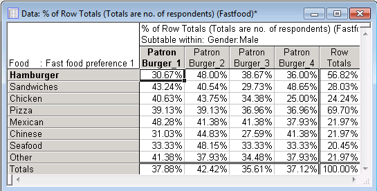
Look at the two-way Food by Patron table for Males:
30.67% of all male respondents who listed Hamburger as either their most favorite, second favorite, or third favorite fast food had eaten at Burger Meister in the two weeks prior to the survey; 48.00% had eaten at Bill's Best Burgers, and so on. After reviewing the percentages in this table, it appears that Male subjects, regardless of stated fast-food preference, generally were more likely to have eaten at Bill's Best Burgers recently (with the exception of the Mexican food row).
In the sub-table for Females, no such simple pattern is apparent (however, note that those percentages are based on few observations, i.e., 36 females).
Concluding remark. If you are not familiar with multiple response variables and dichotomies (factors), it may at first seem somewhat complicated to interpret the frequency or crosstabulation tables of such variables. The best way to verify that one understands the way in which the respective tables are constructed is to crosstabulate some simple example data, and then to trace how each case is counted.
See also, the Basic Statistics and Tables Index and Overviews.

