Example 2: Regression Tree for Predicting Poverty
This example is based on a reanalysis of the data presented in Example 1: Standard Regression Analysis for the Multiple Regression module. It demonstrates how regression trees can sometimes create very simple and interpretable solutions.
- Data file
- The example is based on the data file Poverty.sta. Open this data file via the File - Open Examples menu; it is in the Datasets folder. The data are based on a comparison of 1960 and 1970 Census figures for a random selection of 30 counties. The names of the counties were entered as case names.
The information shown below for each variable is displayed in the Variable Specifications Editor (accessible by selecting All Variable Specs from the Data menu).
- Research question
- The purpose of the study is to analyze the correlates of poverty, that is, the variables that best predict the percent of families below the poverty line in a county. Thus, you will treat variable 3 (Pt_Poor) as the dependent or criterion variable, and all other variables as the independent or predictor variables.
Setting up the analysis. With one exception (V-fold cross-validation), we will use the default analysis options in the General Classification and Regression Trees Models (GC&RT) module. Select this command from the Data Mining menu to display the Startup Panel. Select Standard C&RT as the Type of analysis (i.e., accept the default) and click OK to display the Standard C&RT Specifications dialog. On the Quick tab, click the Variables button and select PT_POOR as the dependent variable, and all others as the continuous predictor variables. Do not select the Categorical response option in this example, as PT_POOR (percent of families below poverty level) contains continuous data.
Next click on the Validation tab and select the V-fold cross-validation check box. As described in the Introductory Overview, this option is particularly useful in cases when the data file is not very large to derive a more stable estimate for the right-size tree. Next click OK to begin the analysis; the progress of the computations are indicated in a Computing... dialog, and then the GC&RT Results dialog will be displayed.
- Reviewing Results
- Click the Tree graph button on the
Results dialog - Summary tab.
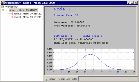
The solution appears to be very simple and straightforward. Click the Tree browser button to further review the details of the solution: The Workbook Tree Browser (see Reviewing Large Trees: Unique Analysis Management Tools in the Introductory Overview - Basic Ideas Part II) summarizes the tree as well as the split conditions and (classification) statistics for each splitting (intermediate) node (indicated by
 ) or terminal node (
 ).
).
One of the useful features of the Workbook Tree Browser (see also General Computation Issues and Unique Solutions of STATISTICA C&RT in Introductory Overview - Basic Ideas Part II) is the ability to review "animations" of the final solution. Start by highlighting (clicking on) Node 1. Then use the arrow keys on your keyboard to move down the nodes of the tree. You can clearly see how the consecutive splits produce nodes of increasing purity, i.e., homogeneity of responses as indicated by the smaller standard deviation of the normal curve.
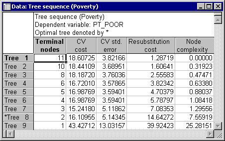
We will interpret the results shown in this tree in a moment; but next click the Tree sequence button on the Summary tab.
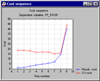
Tree number 8 is the least complex tree (least number of terminal nodes) with the lowest cross-validation cost (CV cost); hence it was selected as the "right-size" tree. Click the Cost sequence button to display these results in a graph.
Note how the Resubstitution cost for the sample from which the splits were determined increases as the pruning proceeds (note that as the tree number increases from 1 to 10, the number of terminal nodes decreases, i.e., consecutive tree numbers are increasingly "pruned-back"); this is to be expected since the fit for the data from which the tree was computed will become worse the fewer terminal nodes are included. However, interestingly, the CV (cross-validation sample) cost at first decreases, and clearly "bottoms-out" at tree number 8, indicating that trees 1 through 7 may actually "over-fit" the data, i.e., produced results that were so specific to the sample from which the splits were computed that they led to decreased prediction accuracy in the cross-validation samples (successive v-folds, i.e., randomly drawn cross-validation samples).
It is hard to overestimate the importance of the V-fold cross-validation tool (see the description of this option in Quick specs dialog - Validation tab) for determining and evaluating the "right-size" tree. Without it, in particular in small to moderately sized data sets, it is otherwise very difficult to perform the proper pruning to avoid overfitting of the data and to produce a "good" tree for prediction.
- Interpreting the Results
- Since it looks like the final tree (tree number 8) is, indeed, the "right-size" tree for these data, what do these results tell us about the prediction of poverty in the 30 counties? Return to the
Workbook Tree Browser; there is 1 split nodes (splitting conditions):
If variable PT_PHONE (Percent residences with telephones) is less than 72, the poverty rate appears to be higher; the means are 29.62 vs. 19.18 if this condition is met (PT_PHONE<72), vs. when it is not met (PT_PHONE>=72). This result makes sense: Those counties that are generally more affluent and less poor have more households with phones.
However, these results are easy to summarize and report, and interestingly, also not entirely consistent with the results reported in Example 1: Standard Regression Analysis for the Multiple Regression module.


