Response Optimization Technical Notes

The Simplex Search Algorithm

The Simplex [R. O'Neil (1985)] search technique is a nongradient-based optimization algorithm used for minimizing (or maximizing) an arbitrary function in a finite number of iterations. The algorithm works for any number of continuous independent variables and makes no assumptions about the nature of the function that we need to optimize, except that it is continuous. The algorithm starts with an initial solution and tests its optimality (its closeness to the desired response value subject to the search constraints). If the optimality is satisfied, the algorithm terminates. Otherwise, the algorithm identifies another optimal point by drawing a simplex. The optimality of this new solution is then tested, and the entire scheme is repeated until an optimal set of independent values is found for which the model yields the desired response.

When using the Simplex algorithm for response optimization, it is recommended that you confine your search to those regions of independent space falling within the boundaries of the data set for which the models were trained. That is, of course, unless you have reasons not to. Making predictions in regions of independent space substantially lying outside the boundaries of the data set used to train the model may lead to unreliable results (see Extrapolation below).

The Grid (Exhaustive) and Random Search Algorithm

The Grid and Random search techniques are unguided algorithms based on brute computing power. Hence, they can be computationally more expensive than the Simplex algorithm but, nevertheless, they are useful as alternative tools if the Simplex did not yield the desired results. There are no assumptions behind the applications of these algorithms and, thus, they cannot fail.

The Grid and Random algorithms work in similar ways. They simply take samples from the space of the independent variables. For each sample, the model predictions is computed and compared with the best value found from the previous iterations. If the newly found value is better than the previous one, the new results are stored. This process is repeated until the end of iterations is reached.

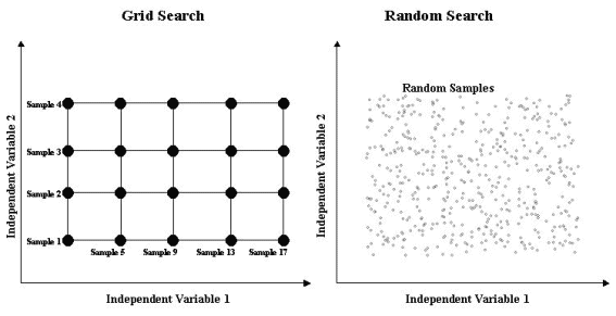
The Grid algorithm performs the sampling by partitioning the space of the independent variables into a grid scheme, with the boundaries of the grid determined by the start and end values for the independent variables (see schematic below). The intensity of the computation is determined not only by the start and end values but also by the size of the steps used to forward the search from one location of the independent space to another.

In contrast, the Random algorithm samples from the space of the independent variables by randomly drawing samples according to a uniform distribution with a given mean and variance.

When using the Grid or Random algorithm for response optimization, it is recommended that you confine your search to those regions of independent space falling within the boundaries of the data set for which the models where trained, unless you have reasons not to. Making predictions in regions of independent space substantially lying outside the boundaries of the data set used to train the model may lead to unreliable results (see Extrapolation below).

Model Exploration

Although the main functionality of STATISTICA Response Optimization for Data Mining Models is to find a set of independent values for which the predictive models yield the desired responses, the use of this module is by no means restricted to this type of analysis. You can use the Response Optimization module to explore model responses calculated at any particular set of values for the independent variables. This enables you to explore your predictive models and observe their behavior when one independent variable takes different values while the rest are fixed .

Model exploration is a continuous form of the What if analysis. While one specially chosen independent variable is altered and fixed values are provided for the other independent variables of the predictive model(s), the response of the predictive model is calculated and the results are presented in the form of convenient spreadsheets and graphs. In other words, the Model exploration feature enables you to monitor the behavior of the response for your predictive model in a one-dimensional slice through an N dimensional response surface, where N is the number of independent variables.

If more than one model is present in your analysis, the response graphs and spreadsheets also includes responses for the combined models (i.e., ensemble predictions) together with their error bars (for continuous dependents only). The error bars measure the extent of the agreement (or disagreement) among the predictive models (see Extrapolation below).

Extrapolation

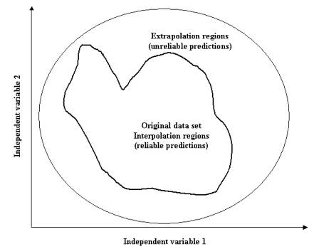
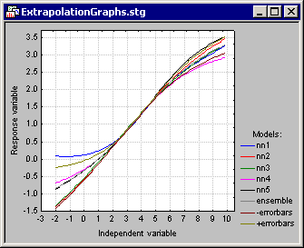
Given a predictive model, it is often necessary to estimate predictions for some other arbitrary points that weren't included in the training data set. Such predictions are called extrapolation. Making predictions at locations of independent space falling well outside the boundaries of the data set used to train the predictive model should be handled with care. In such regions model predictions may become unreliable. In fact, predictions may substantially vary from one model to another even if the models were trained on the same data set. As an example, the above figure shows several neural network models trained on a data set consisting of one dependent and one independent variable. The observed minimum and the maximum of the independent variable in the training data set were within 1.1 to 6.9, respectively. Note that in this interval the predictions of the model are in good agreement. However, outside this region the models increasingly differ. As a result, the combined models (i.e., the ensemble) have large error bars indicating this disagreement.

Ensemble of Predictive Models

Ensembles (i.e., a committee of predictive models) are collections of predictive models that cooperate in making predictions for the dependent (response) variable given a set of independent values. The STATISTICA Response Optimization for Data Mining Models module supports this type of model predictions for performing response optimization.

It is sometimes common practice to train a number of different models (e.g., Support Vector Machines, MARSplines, Trees, Neural Networks, etc.) on the same data set, and then select the model that performs best on a test set. The problem with this approach is that the performance on the test set has a random component, i.e., the model may perform well on the test set, yet perform badly on another validation set. Such complications can be alleviated using ensembles of predictive models instead of a single model [see Bishop(1995) for further details]. It is often the case that the performance of an ensemble is better than the single best predictive model given the same test or validation data set (a validation data set is a new data set, such as the test set, which was not used to train the predictive model).

In making predictions, an ensemble estimates a value for the response variable by combining the individual responses. Thus, if an ensemble involves a Support Vector Machine (SVM), a MARSplines (MAR), and a Neural Network (NN) model, the response ENSEMBLE of the ensemble is given by the linear average

where SVM is the response of the Support Vector Machine, MAR is the response of the MARSplines model, and NN is the response of the Neural Network. For regressions tasks, the response is simply the prediction of the predictive model, while for classification tasks, the response is the classification confidence. Given the above, the variance of an ensemble is

and its errorbars are