Models and Methods - The SEPATH Model
Let mx be a vector of manifest exogenous variables. Partition the variables into vectors s1 and s2 as follows:
 (34)
(34)
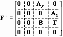
and
![]() (35)
(35)
Then one may write
s1 = Bs1 + Gs2(36)
where
 (37)
(37)
and
 (38)
(38)
Assuming a nonsingular I - B, Equation 23 may be rewritten as
s1 = (I - B)-1Gs2.(39)
Let G be a filter matrix which extracts the manifest variables from s1, and let X = E(s2s2¢ ) be the covariance matrix for s2.
Then
![]() (40)
(40)
and one obtains the following model for covariance structure:
S = G(B - I)-1GXG¢ (B¢ - I)-1G¢ (41)
The covariance matrix Cov (s1) = Y for manifest exogenous, manifest endogenous, and latent endogenous variables may be computed as
Y = (B - I)-1GXG¢ (B¢ - I)-1(42)
The model of Equation 41 allows direct correspondence between all permissible PATH1 statements and the algebraic model. There is no need to concoct dummy latent variables. All possible types of relationships among manifest and latent variables are accounted for. After a model is complete, all variables can immediately be assigned to one of the 4 vectors mn, mx, ln, or lx. All coefficients (for arrows) are then assigned to the matrices F1 through F8. The column index for a variable (in any of these 8 matrices) represents the variable from which the arrow points, the row index the variable to which the arrow points. Coefficients for wires are represented in a similar manner in the matrix X.
The model of Equation 41 sacrifices some of the simplicity of the RAM model, because variables must be assigned to 4 types before the location of model coefficients can be determined. However, in our typology and with the SEPATH diagramming rules the typing of each variable into one of 4 categories can be determined by looking only at that variable in the path diagram. Because two headed arrows are eliminated, a variable is endogenous if and only if it has an arrowhead directed toward it. A variable is latent if and only if it appears in an oval or circle. (If it is not already obvious, let us note that with two headed arrows one must look away from the variable of interest to determine if the variable is endogenous, because an arrowhead attached to the variable and pointing to it might be two-headed! Not only is the SEPATH system less cluttered, but it is also visually more efficient.)
Two final points should be emphasized. First, it is not clear which of the above models is, in any overall sense, "superior" to the others. The SEPATH model of Equation 41 was chosen primarily because it offered a good trade-off between certain conceptual and computational advantages. However, there are also definite advantages, both conceptual and computational, in each of the other model formulations.
Second, it is possible to express some of the models as special cases of the others. For example, the LISREL model can be written easily as a COSAN model. To see why, suppose that the manifest and latent variables were ordered in the v of Equation 10 so that
![]() (43)
(43)
Then it follows immediately that one may write v = F*v + r* where
 (44)
(44)
and
![]() (45)
(45)
If P* is defined as the covariance matrix of r*, then clearly one can test any LISREL model as a COSAN model of the form
S = G (F* - I)-1 P (F¢ * - I)-1G¢ (46)
where G is a matrix which filters x and y from v.