Example 3: Aligning Multiple Stages of Process Data
Overview
Pharmaceutical companies have been tasked by the United States Food and Drug Administration (FDA) to model the relationship between their manufacturing processes and outcomes for quality purposes. This framework is referred to as Process Analytical Technology.
Process data (multiple temperatures, multiple pressures, etc.) recorded in frequent intervals (e.g., every minute) at different stages of the manufacturing process from an automated control system flow directly to sensors and are entered into a data historian such as OSIsoft's PI System or Wonderware.
Also, it is somewhat typical to have 1-10 (or, at the very most, 20) instances of product quality measures. These measures include both in-process (taken periodically throughout the process) and finished product tests (taken at the end of the process) on samples from a particular batch. This quality data is typically stored in a relational database such as a Laboratory Information Management System (LIMS).
As a result, a pharmaceutical company may have two different databases on two different servers, which may be in different locations. Before analyzing the relationship between the manufacturing process and how it relates to product quality outcomes, statisticians need a way to meld the two types of data.
In this example, ID-Based STATISTICA ETL is used to line up data from disparate sources by batch number. Merging many-to-one data sets is a common scenario in the pharmaceuticals industry.
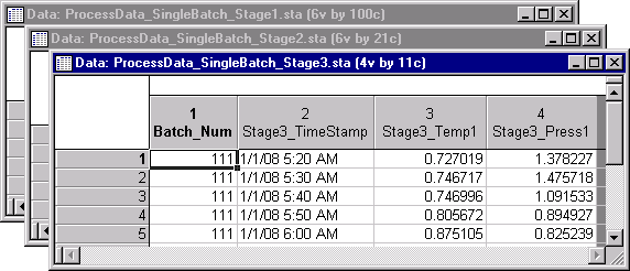
This example is based on four data sets, which are included with STATISTICA. Each data set contains a batch number, a date-time stamp, and various measures. Each data set contains only one batch so that it is easier to see how data sets are merged and aligned.
Starting the analysis
- Ribbon Bar: Select the Home tab. In the File group, from the Open menu, select Open Examples to display the Open a STATISTICA Data File dialog box. Double-click the Datasets folder, and then open the four data sets. Then, on the Home tab, in the File group, click Open - Open External Data - Extract, Transform, and Load (ETL) - ID-based and Batch Data to display the STATISTICA Extract, Transform, and Load (ETL): ID-Based Startup Panel. (This analysis can be accessed from the Data tab, Transformations group as well.)
- Classic menu: Open the data files by selecting Open Examples from the File menu to display the Open a STATISTICA Data File dialog. The data files are located in the Datasets folder. Then, from the submenu, select ID-based and Batch Data to display the STATISTICA Extract, Transform, and Load (ETL): ID-Based Startup Panel. (This analysis can be accessed from the Data menu as well.)
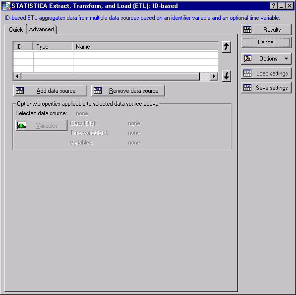
- The Startup Panel contains two tabs:
Quick and
Advanced.
The Quick tab displays the most commonly used options such as data source and variable selection.
The grid at the top of the tab will list the selected data sources and their associated properties such as data source ID (for recording/editing SVB macros), data type, and name. Use the arrows to the right of the grid to change the sequence in which the data sources are aligned/merged.
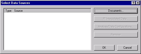
- Click the Add data source button to display the Select Data Sources dialog box.
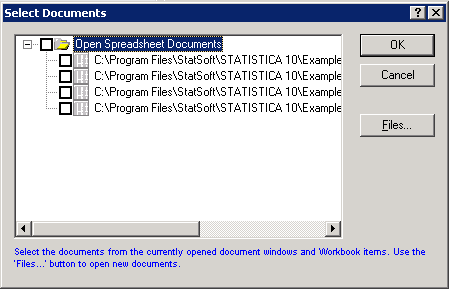
- Click the Documents button to display the Select Documents dialog box. The four files previously opened are listed. Alternatively, you can select these files through this dialog box by clicking the Files button.
- Documents can be selected from the list by clicking the individual check boxes adjacent to each file. Since this example uses all displayed files, select the Open Spreadsheet Documents check box at the top of the list to select all four data files, and then click the OK button.
- Click the
OK button in the
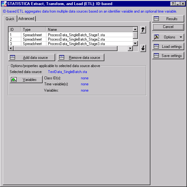
Select Data Sources dialog box to add the files to the analysis. The
Quick tab on the
STATISTICA Extract, Transform, and Load (ETL): ID-based dialog box appears.
Now that we have selected data sources, the next step is to select variables. ID-based STATISTICA ETL aggregates data from multiple data sources based on an identifier variable (either number or text) and an optional time variable.
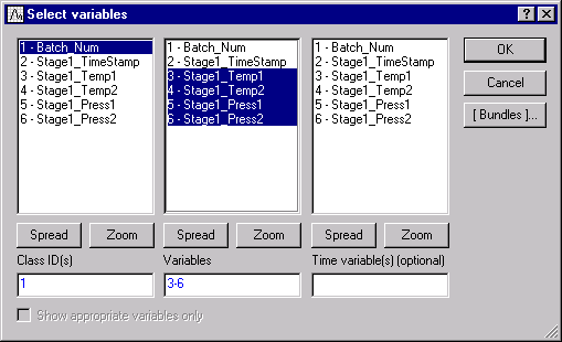
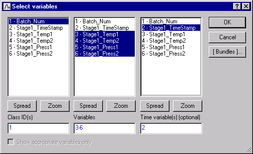
- We first aggregate data using only an identifier variable. In the grid, select the first data source, ProcessData_SingleBatch_Stage1.sta, and click the Variables button to define variables to be included in the output. In the first pane, select Batch_Num for the Class ID variable. In the second pane, select Stage1_Temp1, Stage1_Temp2, Stage1_Press1, and Stage1_Press2 for the output variables.
- Click the OK button.
- We now move on to other three data sources. For ProcessData_SingleBatch_Stage2.sta, select variables as follows. In the first pane, select Batch_Num for the Class ID variable. In the second pane, select Stage2_Temp1, Stage2_Temp2, Stage2_Press1, and Stage2_Press2 for the output variables. Click the OK button.
- For ProcessData_SingleBatch_Stage3.sta, select variables as follows. In the first pane, select Batch_Num for the Class ID variable. In the second pane, select Stage3_Temp1 and Stage3_Press1 for the output variables. Click the OK button.
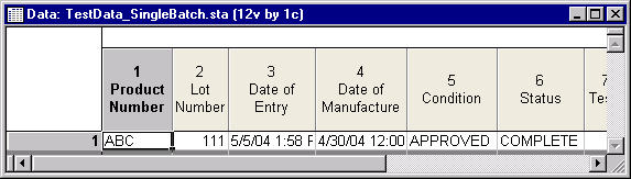
- Scroll the list to see the last data source in the list view. For TestData_SingleBatch.sta, select variables as follows. In the first pane, select Lot Number for the Class ID variable. In the second pane, select Condition, Status, Test1, Test2, Test3, Test4, Test5, and Test6 for the output variables. Click the OK button. Variables have now been selected for all four data sources.
Reviewing the results
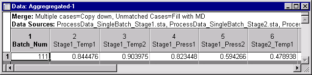
- Click the Results button to create a results spreadsheet aligned by a Class ID variable. The many rows of process data are aggregated into one row of computed means. Meanwhile, the one row of quality control data is left unchanged. The resultant spreadsheet contains a single row of data aligned by the Batch_Num variable.
- This example demonstrates a many-to-one merge for a batch. Let's say that more than one row of resultant data is desired for a batch. We aggregate data using both an identifier variable and a time variable. With a time variable selected, data may be optionally aligned by N-equal intervals or N-user-specified intervals.
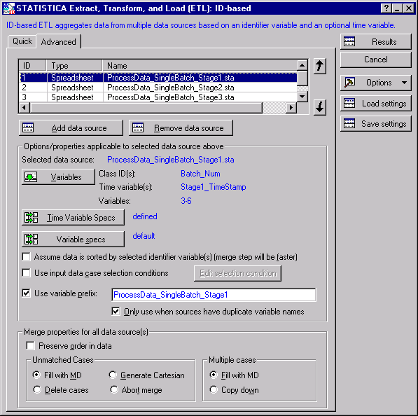
- Select the Advanced tab to display the same options as on from the Quick tab, plus additional options such as Time Variable Specs button, Variable Specs button, data source check boxes, and Merge properties.
- Note that the Time Variable Specs button is disabled.
- Select the first data source ProcessData_SingleBatch_Stage1.sta and click the Variables button to redefine variables.
- In the third pane, select TimeStamp for the time variable.
- Click the
OK button to return to the
Advanced tab.
Adjacent to the Variables button, blue text now displays a time variable, Stage1_TimeStamp, for the selected data source ProcessData_SingleBatch_Stage1.sta. In addition, the Time Variable Specs button is now enabled.
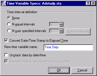
- Click this button to display the Time Variable Specs dialog.
- This dialog provides the following options:
- Normalize the lengths of batch data to achieve a fixed number of time intervals for all batches in the respective input data source
- Optionally unstack the batch-time data. For each time interval and for each output variable, a new variable is created. This prepares data for Multivariate Statistical Process Control (MSPC)
The Time interval definition group box provides three data alignment options. The default option is None, which retains all date/time stamps and retains existing batch sizes. Select the N-equal intervals option button. The text field beside the option button displays a default of 5. This setting divides every batch into 5 equal time intervals using the empirical distribution function with averaging percentile method. You could change the setting from 2 to 100 intervals, but keep the default of 5 for this example.
Below the Time interval definition group box are three check boxes. Keep the defaults for each of these. The selected Convert Date/Time Stamp to Elapsed Time check box creates a new time-based column with discrete interval values (i.e., 0, 1, 2, 3, etc.) in the results spreadsheet; the new Time Step column can be used by Multivariate Statistical Process Control (MSPC) to determine trends in the evolution of process variables
- Since the data is already unstacked, leave the Unstack data by date/time check box cleared.
- Click the OK button, to return to the STATISTICA ETL: ID-Based - Advanced Tab.
- Click the Variable specs button to display the
Variable Specification dialog box.
The Variable Specification dialog box provides options for each selected output variable (e.g., Stage1_Temp1, Stage1_Temp2, Stage1_Press1, and Stage1_Press2). The first two columns, Minimum permissible value and Maximum permissible value, are for data cleaning of continuous variables. Assuming there is a known issue with one of the pressure data sensors, enter a minimum value of 0.1 for variable Stage1_Press2. This converts any value less than 0.1 to missing data. The last column, Aggregation statistics type, summarizes data by central tendency, variation, range, total, or none.
- Since the default is Mean, output variables are averaged. Leave the default values and click the OK button.
- Below the Variables Specs button are several check boxes: (1) Assume data is sorted..., (2) Use input data case selection conditions, and (3) Use variable prefix. The default settings are correct for this example, so leave the defaults as they are.
Merge properties for all data sources are listed the bottom of the dialog box. By default, the Preserve order in data check box is cleared; this merges results, and are sorted in the ascending order on the basis of the Class ID variable. The Unmatched cases options specify how unequal numbers of cases are handled; the default Fill with MD option pads unmatched cases with missing data. The Multiple cases options specify how duplicate matching cases are handled; the default Fill with MD option pads duplicate matched cases with missing data. The default settings are correct for this example, so leave the defaults as they are.
- Set time properties for the other data sources as follows.
- Select ProcessData_SingleBatch_Stage2.sta.
- Click the Variables button, select TimeStamp for the time variable, and click the OK button.
- Click the Time Variable Specs button, select the N-equal intervals option button, and click the OK button.
- Repeat the same Time Variable Specs and Variable Specs selections for ProcessData_SingleBatch_Stage3.sta. No changes are needed for TestData_SingleBatch.sta since it contains only one row of data.
- Click the
Results button to create a results spreadsheet aligned by Class ID and Time variables.
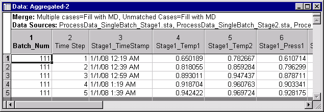
The resultant spreadsheet contains five rows of data aligned by Batch_Num. In this example, process measures (e.g., temperature and pressure) are aggregated into five equal intervals as means. Quality measures are left unchanged and repeated five times to match up with the process data.
Now that process data has been aligned with quality data in a fixed number of elapsed time intervals (i.e., normalized batch lengths), you can analyze time-dependent changes against static quality outcomes with STATISTICA Multivariate Statistical Process Control (MSPC). MSPC implements two statistical multivariate data analysis techniques known as Principal Component Analysis (PCA) and Partial Least Squares (PLS).

STATISTICA PCA
It is a mathematical procedure that aims to represent a set of (possibly correlated) multivariate variables with the aid of a smaller number of uncorrelated variables known as principal components. In other words, it is a multivariate projection method designed to extract systematic variation and relationships among the variables of a data set. This transformation (projection) often simplifies the analysis at hand while also alleviating the worse symptoms of high dimensionality, which is present when the number of variables is large. This makes PCA an ideal technique for solving problems when we are typically faced with a large number of predictor variables.
Other important applications of PCA include data diagnostics, both on observation and variable levels. The observation level helps us to detect outliers, while the variable level provides us with insight of how the variables contribute to the observations and relate (correlate) to one another. These diagnostic features of STATISTICA PCA are particularly useful for process monitoring and quality control as they provide us with effective and convenient analytic and graphic tools for detecting abnormalities that may rise during the development phase of a product. PCA data diagnostics also play an important role in batch processing where the quality of the end product can only be ensured through constant monitoring during its production phase.
STATISTICA PLS
It is a popular method for modeling industrial applications. It was developed by Herman Wold in the 1960s as an economic technique, but soon its usefulness was recognized by many areas of science and engineering including multivariate statistical process control in general and chemical engineering in particular. Although the PLS technique is primarily designed for handling regression problems, STATISTICA PLS also enables you to handle classification tasks. You can find this dual capability useful in many applications of regression or classification, especially when the number of predictor variables is large.
For more information,see also Multivariate Statistical Process Control Startup Panel and Quick Tab.