Developing Credit Scoring Model for Data Miner Recipe - Example
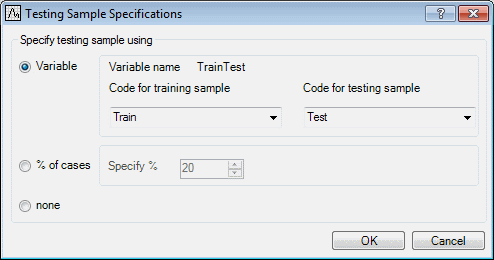
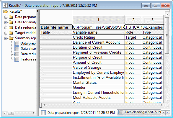
The purpose of this example is to explore the use of Statistica Data Miner Recipes for Credit Scoring applications. The example is based on the data file CreditScoring.sta, which contains observations on 18 variables for 1,000 past applicants for credit. Each applicant is rated as good credit (700 cases) or bad credit (300 cases). We want to develop a credit scoring model that can be used to determine if a new applicant is a good credit risk or a bad credit risk, based on the values of one or more of the predictor variables. An additional Train/Test indicator variable is also included in the data file for validation purposes.
Procedure
Nodes (steps)
 indicates a wait state, meaning a step cannot be started because it is dependent on a previous step that has not been completed; a yellow
 indicates a ready state, meaning you are ready to start the step because previous steps have been completed; a green
 indicates a completed step. To change the yellow
(ready state) to the green
(completed state), click the
Next step button . The change is made only if the step is successfully completed.
indicates a completed step. To change the yellow
(ready state) to the green
(completed state), click the
Next step button . The change is made only if the step is successfully completed.
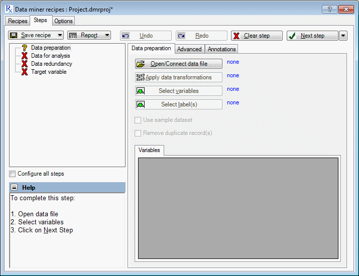
Preparing Data Step for Data Miner Recipe
Procedure
-
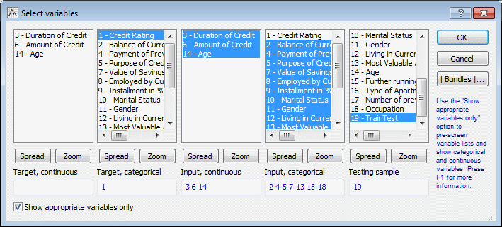
Click the
Select variables button. In the Select variables dialog box, select the
Show appropriate variables only check box. Then, select:
- Variable 1 (Credit Rating) as the Target, categorical variable,
- Variables 3, 6, and 14 as Input, continuous (continuous predictors)
-
To ensure that the step is successfully completed (in the step-node panel next to
Data preparation, the yellow
changes to a green
), click the
Next step button for the
Data preparation step.
Analyzing Data Step for Data Miner Recipe
Eliminating Data Redundancy Step for Data Miner Recipe
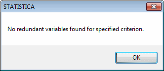
After the Data for analysis step is completed, the Data redundancy step is selected. The purpose of the Data redundancy step is to eliminate highly redundant predictors. For example, if the data set contained two measures for weight, one in kilograms the other in pounds, those two measures are redundant.
Procedure
Target Variable Step for Data Miner Recipe
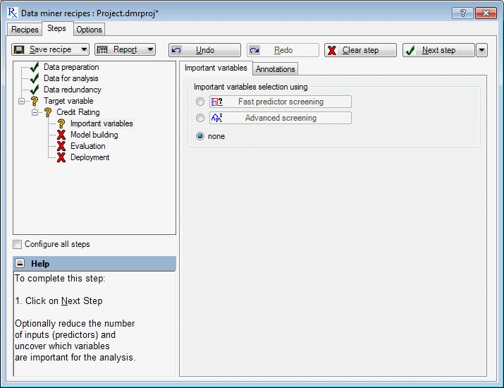
Selecting Important Variables for Target Variables Step
The Important variables node is selected automatically. In this step, the goal is to reduce the dimensionality of the prediction problem, to select a subset of inputs that is most likely related to the target variable (in this example, Credit rating) and, thus, is most likely to yield accurate and useful predictive models. This type of analytic strategy is also sometimes called feature selection.
Two strategies are available. If the Fast predictor screening option button is selected, the program screens through thousands of inputs and find the ones that are strongly related to the dependent variable of interest. If the Advanced screening option button is selected, tree methods are used to detect important interactions among the predictors.
Procedure
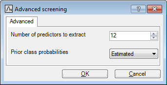
- To display the Advanced screening dialog box, click the Advanced screening button. Enter 12 in the Number of predictors to extract field.
- To review a summary of the analysis thus far, on the Steps tab, click the Report button, and from the drop-down list, select Summary report to display the Results workbook.
Building Models for Target Variables Step
The Data miner recipe dialog box is minimized so that the Results workbook dialog box is visible. To display the dialog box again, click the Data miner recipes button located on the Analysis Bar at the bottom of the application.
Next, the Model building node is selected. In this step, you can build a variety of models for the selected inputs.
On the Model building tab, the C&RT, Boosted tree, and Neural network check boxes are selected by default as the models or algorithms that are automatically be tried against the data.
The computations for building predictive models are performed either locally (on your computer) or on the Statistica Enterprise Server. However, the latter option is available only if you have a valid Statistica Enterprise Server account and you are connected to the server installation at your site.
For this example, to perform the computations locally on your computer, click the Build model button. This takes a few moments; when finished, click the Next step button to complete this step.
Evaluating and selecting models for Target Variables
Procedure
-
Now, the Evaluation node is selected. To perform the competitive evaluation of models for identifying the best performing model in terms of performance in the validation sample, on the
Evaluation tab, click the
Evaluate models
button.
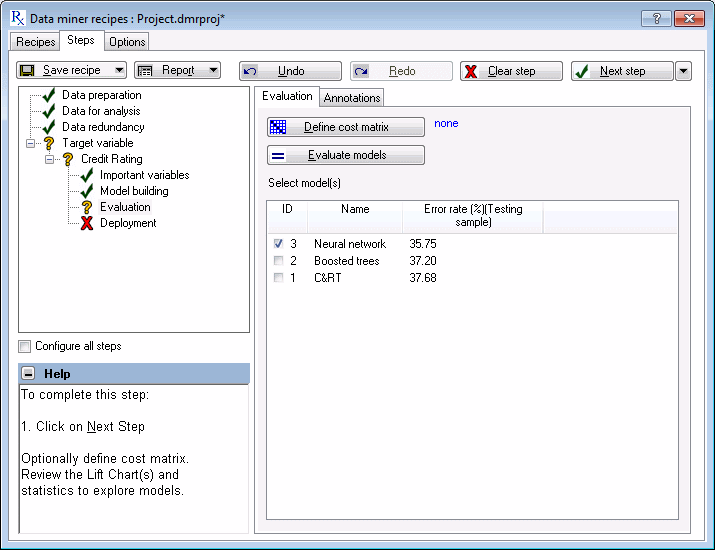
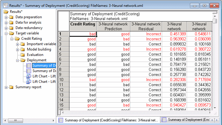
Notice that the Neural network model has the minimum error rate of 35.75% (exact results may vary). In other words, 64.25% of the cases in the validation sample are correctly predicted by this model. Your results (the best model and the percentages) might vary because these advanced data mining methods randomly split the data into subsets during training to produce reliable estimates of the error rates.
Deploying for Target Variables Step