Example 1: Variance Component Estimation for a Two-Way Random Factorial Design
- Specifying the Design
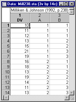
- This example is based on a small data set presented in Milliken and Johnson (1992, p. 238). The dependent variable is DV and the random factors are A and B. The data are shown below and are available in the mill238.sta data file. Open this data file via the File - Open Examples menu; it is in the Datasets folder.
Milliken and Johnson (1992) first analyzed this data set using a two-way factorial ANOVA treating both factors and their interaction as random effects. To perform this analysis, select Variance Components from the Statistics - Advanced Linear/Nonlinear Models menu to display the Variance Components & Mixed Model ANOVA Startup Panel. On the Quick tab, click the Variables button to display the standard variable selection dialog. Here, select variable DV as the Dependent vars, variables A and B as Random factors, and then click the OK button. By default, a full factorial design will be created, with the A by B interaction treated as a random effect, so click the OK button to display the Variance Components and Mixed Model ANOVA/ANCOVA Results dialog.
Reviewing the Results.
- ANOVA Estimation of Variance Components - Type I estimates
- One method that Milliken and Johnson (1992) used to estimate the variance components for the dependent variable was the ANOVA-based Type I
Expected mean squares (MS) Method. Click on the
Advanced tab on the
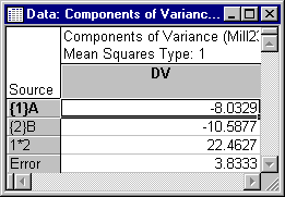
Results dialog. As you can see under Method and SS Type, this is the default method, so simply click the Summary: Components of variance button to display three spreadsheets; we will look at the Components of Variance spreadsheet, shown below.
Within rounding, these estimates agree with those presented by Milliken and Johnson (1992, p. 239).
- ANOVA Estimation of Variance Components - Type III estimates
- Milliken and Johnson (1992) also estimated the variance components using Type IV sums of squares. Type IV estimates for data without missing cells correspond to Type III estimates, so select the Type III option button under SS Type, and then click the Summary: Components of variance button on the
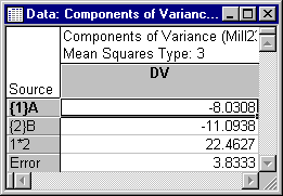
Advanced tab to display three spreadsheets; we will once again look at the Components of Variance spreadsheet, shown below.
Again, these estimates agree with those presented by Milliken and Johnson (1992, p. 239). Note that for both sets of estimates, the variance components for A and B are estimated to have negative values. This is one of the disconcerting features of variance component estimation; estimates are quite often negative. In practice, negative variance components are usually treated as indicating a 0 (zero) component, and thus are not necessarily problematic. Therefore, both sets of estimates clearly agree in suggesting that the A by B interaction effect represents the only nonzero component of variance in the dependent variable (other than Error).
To test the significance of random effects, error terms must be constructed that contain all the same sources of variation except for the variation of the respective effects of interest. This is done using Satterthwaite's method of denominator synthesis (Satterthwaite, 1946), which finds the linear combinations of sources of variation that serve as appropriate error terms for testing the significance of the respective random effects. The Denominator Synthesis: Coefficients spreadsheet is one of the optional spreadsheets that can be requested by selecting the Coefficients for denominator synthesis check box below the Summary: Components of variance button. Clicking the Summary: Components of variance button will then display one additional spreadsheet, the Denominator Synthesis: Coefficients spreadsheet along with the other previously displayed spreadsheets. The Denominator Synthesis: Coefficients spreadsheet displayed below shows the coefficients used to construct the linear combinations of sources of variation based on Type I Expected mean squares (MS) Method for the mill238.sta data set (therefore, before you click the Summary: Components of variance button, select the Type I option button under SS Type).
The coefficients show, for example, that the Mean square for A should be tested against .03125 times the Mean square for B, plus 1.043155 times the Mean square for the A by B interaction, minus .074405 times the Mean square for Error. To perform the tests of significance of the random effects, ratios of appropriate Mean squares are formed to compute F statistics and p-values for each random effect. The ANOVA Results for Synthesized Errors spreadsheet is another optional spreadsheet that can be requested by selecting the Denominator synthesis ANOVA check box below the Summary: Components of variance button (by default it is already checked). The ANOVA Results for Synthesized Errors spreadsheet is displayed below (for the Type I Expected mean squares (MS) Method).
As shown in the spreadsheet, the A by B interaction effect is found to be significant at p < .05, but neither the A main effect nor the B main effect approach significance, F's < 1.0. Note also that the A and B main effects have fractional denominator degrees of freedom, reflecting the synthesized error terms used to test their effects.
- MIVQUE(0) Estimation of Variance Components
- Milliken and Johnson (1992) also estimated variance components for this data set using the MIVQUE(0) estimation method (see
Variance Components and Mixed Model ANOVA/ANCOVA Method Options). As a preliminary step to performing MIVQUE(0) estimation, it is useful to inspect the Sums of Squares and Cross-Products (SSCP) matrix. So, click on the
Estimation tab of the
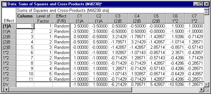
Results dialog and then click the SSCP matrix button to display several spreadsheets, including the Sums of Squares and Cross-Products spreadsheet, a portion of which is shown below.
The elements of the SSCP matrix shown above indicate the variation and covariation among the A and B main effect columns of the design matrix. In the design matrix, there is one column variable for each level of each effect, and cases are coded in these column variables with values of 0 (zero) or 1 (one) to denote non-membership or membership, respectively, in the groups defined by each level of each effect. The SSCP matrix is then produced by premultiplying the design matrix by its transpose (after residualizing it on the intercept, which represents the only fixed effect in this design). The nonzero cross products of some of the A,B elements of the SSCP matrix shown above reflects the covariation between A and B caused by the unbalanced (unequal N) random effects design.
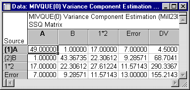
The SSCP matrix is closely related to the Quadratic sums of squares (SSQ) matrix, from which MIVQUE(0) variance components are estimated. Select the MIVQUE0 option button under Method on the Advanced tab and then click the Summary: Components of variance button to display the MIVQUE(0) Variance Component Estimation SSQ Matrix spreadsheet and the MIVQUE(0) Estimation Variance Components spreadsheet, the first of which is shown below.
The elements of the SSQ matrix can most simply be described as the sums of squares of the sums of squares and cross products for each random effect in the model (after residualization on the fixed effects). For example, the value of 49.00000 for the A,A element in the SSQ matrix above is the sum of squares of the elements in the A,A partition of the preceding SSCP matrix (i.e., 49 = 3.52 + 3.52 + 3.52 + 3.52). Nonzero off-diagonal elements in the SSQ matrix reflect the covariation that is taken into account when variance components are computed.
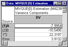
MIVQUE(0) variance components are estimated by inverting the partition of the SSQ matrix that does not include the dependent variable (or finding the generalized inverse, for singular matrices), and postmultiplying the inverse by the dependent variable column vector. This amounts to solving the system of equations that relates the dependent variable to the random independent variables, taking into account the covariation among the independent variables. The estimates for this data set are displayed in the MIVQUE(0) Estimation Variance Components spreadsheet shown below.
- ML Estimation of Variance Components
- Milliken and Johnson (1992) also reported variance components estimates using the Maximum likelihood (ML) estimation method (see
Variance Components and Mixed Model ANOVA/ANCOVA Method Options). To perform Maximum likelihood estimation for this data set, select the ML option button under Method on the
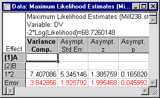
Advanced tab and then click the Summary: Components of variance button to display the Maximum Likelihood Estimates spreadsheet. The variance component estimates displayed in the spreadsheet are shown below.
Within rounding, these estimates agree with those reported by Milliken and Johnson (1992, p. 241). Note that the A by B interaction effect again represents the only nonzero component of variance in the dependent variable (other than Error). The variance component estimates for A and B are 0 (zero), but are not printed by STATISTICA (to improve the readability of the spreadsheet for large designs with many zero components). It is important to recognize that the ML estimates for A and B are 0 (zero), not negative, unlike the estimates produced by MIVQUE(0) estimation. This allows a test of significance for nonzero variance component estimates that would otherwise be inappropriate. Asymptotic (large sample) standard errors, z statistics, and corresponding p-values can be computed for the components with nonzero maximum likelihood estimates at the final iteration (convergence) of the solution (for details, see Searle, Casella, & McCulloch, 1992). The tests of significance displayed in the spreadsheet above show that Error is the only statistically significant component of variance. The component of variance for the A by B interaction effect does not differ significantly from zero, p > .05, one-tailed. It should be emphasized that the asymptotic (large sample) tests of significance for REML and ML variance component estimates are based on large sample sizes, which certainly is not the case for the mill238.sta data set.
Further information about the ML estimates is available on the optional spreadsheets that can be requested along with the variance component estimates. Any combination of the three optional spreadsheets can be requested by selecting the respective check boxes below the Summary: Components of variance button. For this example, select all three and then click the Summary: Components of variance button. The first optional spreadsheet displays the Iteration history, which includes the Log likelihood and the variance component parameter estimates at each iteration of the solution. This spreadsheet is shown below.
The second optional spreadsheet displays the Covariance of Parameters matrix, which is the asymptotic (large sample) variance/covariance matrix of the nonzero variance component parameter estimates at the final iteration (convergence) of the solution. This spreadsheet is shown below.
Note: the Asymptotic (large sample) standard errors for nonzero variance components are derived from the diagonal elements of the Asymptotic Variance/Covariance matrix. For example, the Asymptotic standard error of 5.345146 for the A by B interaction effect is the square root of its Asymptotic Variance of 28.57059.The third optional spreadsheet displays the Parameter correlation matrix, which is the asymptotic (large sample) correlation matrix of the nonzero variance components at the final iteration (convergence) of the solution. This spreadsheet is shown below.
The Parameter correlation matrix shows a reasonably low correlation between the parameter estimates for the A by B interaction effect and Error. High correlations between parameter estimates may indicate an ill-conditioned or unstable solution, in which case it might be advisable to drop one of the highly correlated effects from the model.
- REML Estimation of Variance Components
- Restricted maximum likelihood (REML) estimates of variance components were not reported by Milliken and Johnson (1992), but are shown here for completeness. To perform REML variance component estimation for this data set (see
Variance Components and Mixed Model ANOVA/ANCOVA Method Options), select the REML option button under Method and then click the Summary: Components of variance button to display various spreadsheets depending on the selection of check boxes under the Summary: Components of variance button. The Restricted Maximum Likelihood Estimates spreadsheet is shown below.
As can be seen, the REML variance component estimates and tests of significance agree fairly closely with the previous ML estimates and tests of significance. REML differs from ML in that the likelihood of the data for the random effects is maximized separately from the fixed effects, thus REML is a restricted solution. The same optional spreadsheets available with ML variance component estimation are also available when requesting REML estimates, and can be interpreted in a similar manner.
- Summary
- There is a straightforward conclusion to be drawn from the MIVQUE(0), ML, and REML estimates of the variance components for this data; the dependent variable does not have a significant component of variation for factor A, factor B, or their interaction. The ANOVA estimates led to the contradictory conclusion that the dependent variable does have a significant component of variation for the A by B interaction. This discrepancy may largely be explained by the small sample size for this data set; maximum likelihood tests of significance are notorious for their dependency on sample size (see Searle, 1987). For larger, more realistic data sets, greater agreement for the different variance component estimation methods might be expected. The results of the analysis of the simple mill238.sta data illustrate many of the difficulties that are likely to be encountered in estimating variance components. It should be emphasized, however, that with larger, more realistic data sets, more realistic results would be expected (i.e., nonzero variance component estimates might be found).
See also, Variance Components Index.

