PCA Deployment Example

In the PCA Example, the use of Statistica PCA is demonstrated using the real-world data set IndustrialEvaporator.sta for analyzing the evaporation process in drying a wet product. After numerous analyses and conclusion drawing, the PCA model is saved in PMML format for deployment. In this example, we will continue our analysis by using the model for making further predictions.

Open the IndustrialEvaporator.sta data file, and on the Statistics tab, in the Advanced/Multivariate group, click Advanced Models and select NIPALS to display the PCA/PLS dialog box.

Note that, alternatively, in the Advanced/Multivariate group, click PLS, PCA to display the Multivariate Statistical Process Control dialog box.

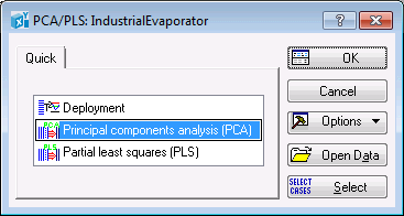
On the Quick tab of the PCA/PLS dialog box, select Deployment and click OK to display the Deployment Model dialog box.

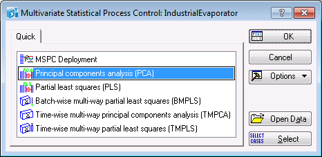
On the Quick tab of the Multivariate Statistical Process Control dialog box, select MSPC Deployment to display the Deployment Model  dialog box.

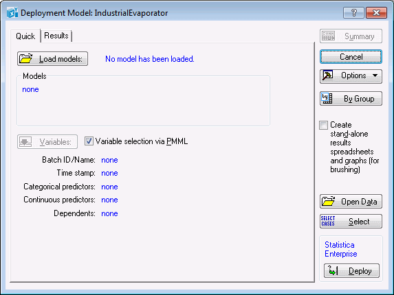
On the Quick tab, click the Load models button to display the Open PMML files dialog box. Select the PCA industrial evaporator.xml file (in a standard installation, located in C\Program Files\Statistica\Statistica *\Examples\Datasets), and click OK. Now you are ready to deploy the loaded model.

By default, variables have been specified via the PMML file and, as part of the model information, also includes the names of the variables that were used in its construction. Alternatively, you can click the Variables button to choose variables from the data set to which the model will be applied. In this example, we will use the default.

NOTE: You can load more than one file in a single analysis, in which case all models will be applied to the same data set one at a time (i.e., you can only generate results for the active mode). A model can be made active by selecting it from the Model drop-down menu on the Results tab.

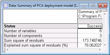
Now you are ready to apply the PC (Principal Component) model to the current data file. First, you may want to review the model by generating a summary spreadsheet: on the Results tab, click the Model summary button.

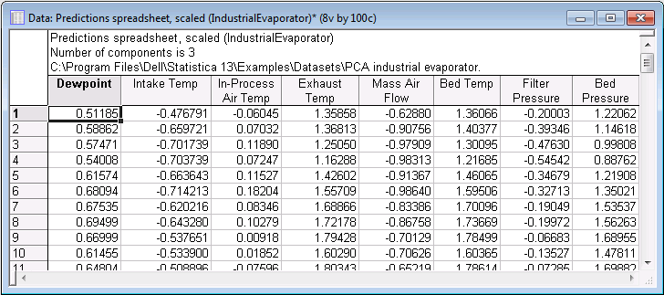
Similarly, you can make predictions for the current data set by clicking the Predictions button in the Results group box on the Results tab.

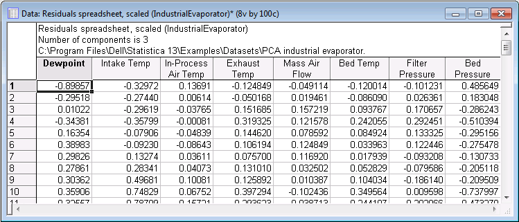
You can also generate a spreadsheet of residuals by clicking the Residuals button. Residuals are the difference between the original data set and the predictions of the PC model. It is that part of the data that could not be explained by the model. Large values of residuals may indicate too simple a model (i.e., a model with an insufficient number of principal components). Alternatively, they might be an indication of the presence of outliers in the original data. The ability to detect outliers is a clear advantage of Principal Components Analysis that can be used for process monitoring and quality control in many areas of industrial research and production. See also, PCA and PLS Technical Notes.

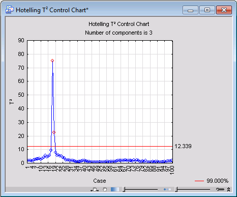
In addition, there are a number of options that you can use to analyze your data further with the aid of the PC model. These options enable you to generate Hotelling T2 and SPE (Q) charts (see PCA and PLS Technical Notes for further details on these charts), which can be used for analyzing the data on a casewise basis. Note that case 18 has a particularly high value of T2, which might well indicate that it is an outlier.

You can also use the options in the Score control chart and summary group box to analyze the data set on a variable-wise basis. For more details, see the documentation for the PCA Results dialog box and the PCA Example.