Principal Components & Classification Analysis Example

This example illustrates how the Principal Components & Classification Analysis module can be used to create a factor space for a set of variables, how to interpret the dimensions, and how to map additional variables and observations into the factor space. The example is based on a data set discussed in Jambu (1991) that contains data for various lifestyle variables (activities) for 28 (groups of) observations.

Specifically, the data describes the numbers of hours spent in each of the 10 activities by 28 different groups of observations. Some of the data are missing, and these data would be substituted by their respective means. Three additional variables, SLEEP, TV, and LEISURE, are considered as supplementary variables. For demonstration purposes (to illustrate how to specify active and supplementary cases) the data were modified to include an additional variable GENDER (for defining active cases), and a variable GEO.REGION for labeling of observations in plots, and so on. Note that because of these additions and modifications to the data, the results from the analyses in this example would not be identical to those reported in Jambu (1991).

Purpose of analysis

The goal of the analysis is to study the relationships among different activities, to derive common dimensions along which one can classify these activities, and to map into those dimensions different population groups.

Specifying the Analysis

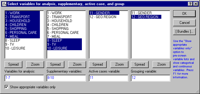
Open the data file Activities.sta, and open the Principal Components & Classification Analysis module through the Statistics - Multivariate Exploratory Techniques submenu. Click the Advanced tab, and then the Variables button to select as Variables for analysis (active variables): WORK through MEAL; Supplementary variables: SLEEP, TV, and LEISURE; Active cases variable: GENDER; and Grouping variable: GEO.REGION.

Also choose FEMALE as the code for active cases in the Code for active cases box. After you have completed the selection of variables, it is important to specify whether the analysis would be based on correlations or covariances; we would base this analysis on the correlation matrix, so select the Correlations option button. Also, in the MD deletion group box, select the Mean substitution option button to substitute the missing values by their respective means.

Reviewing the Results

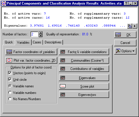
Click OK to perform the initial computations. Then, on the Results dialog set the Number of factors to 2. As a result, the Quality of representation would be computed as 81%.

Let us next review the main results for this analysis: The Summary box at the top of the Results dialog provides useful summary information about the current analysis, such as the number of active and supplementary variables and cases and the eigenvalues. Other results for variables are available on the Variables tab of Results dialog.

Eigenvalues

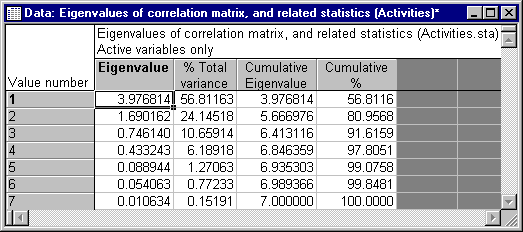
First let us review the eigenvalues; click the Eigenvalues button to produce a spreadsheet with the eigenvalues, percent of total variance, cumulative eigenvalues, and cumulative percent. The eigenvalues in the spreadsheet are arranged in decreasing order, indicating the importance of the respective factors in explaining the variation of the data.

The factor corresponding to the largest eigenvalue (3.976814) accounts for approximately 56.8% of the total variance. The second factor corresponding to the second eigenvalue (1.690162) accounts for approximately 24.14% of the total variance, and so on. When analyzing correlation matrices, the sum of the eigenvalues is equal to the number of (active) variables from which the factors were extracted (computed), and the "average expected" eigenvalue is equal to 1.0. Many criteria are used in practice for selecting the appropriate number of factors for interpretation (see also the Factor Analysis documentation); the simplest is to use (retain for interpretation) as many factors as the number of eigenvalues that are greater than 1. In this example, only the first two eigenvalues are greater than 1, accounting for approximately 81% of total variation.

Scree plot

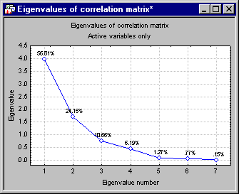
Another method for determining the number of factors to interpret (retain) is to construct the so-called scree plot (Cattell, 1966). Specifically, the successive eigenvalues are shown in a simple line plot. Click the Scree plot button to create this graph.

Cattell suggests to find the place where the smooth decrease of eigenvalues look to level off to the right of the plot. To the right of this point, presumably, one finds only "factorial scree." Scree is the geological term referring to the debris that collects on the lower part of a rocky slope. Thus, no more than the number of factors to the left of this point should be extracted.

Factor coordinates of variables

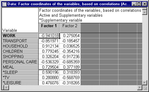
Next, click the Factor coordinates of variables button to display the factor coordinates of the active variables as well as the supplementary variables, for the first two factors. Because the current analysis is based on the correlation matrix, the results displayed in this spreadsheet can be interpreted as the correlations of the respective variables with each factor.

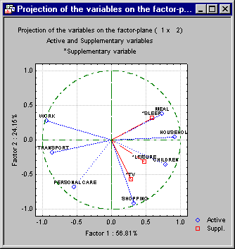
In the current analysis the first axis, corresponding to the eigenvalue 3.976814, is most correlated with the variables WORK and TRANSPORT (high negative correlations), and HOUSEHOLD and CHILDREN (high positive correlations). Based on the magnitudes of the factor coordinates (variable-factor correlations) for the variables in the analysis and the supplementary variables, and the signs of those correlations perhaps one could label the first dimension as Work versus Home related activities (note the high negative coefficients for WORK, TRANSPORT, and PERSONAL CARE versus the positive values for HOUSEHOLD, CHILDREN, and so on) while the second factor may be related to "work-like" (recurrent) activities required by modern organized life (SHOPPING, PERSONAL CARE); however, you may prefer to choose different labels (and the inclusion of additional supplementary variables or cases in future research could clarify the interpretation of the second factor).

Plot of factor coordinates of variables

The plot of factor coordinates often makes the interpretation of factors much easier. Click the Plot var. factor coordinates button to display the factor coordinates for the first two factors.

Note: By default this graph shows a Unit circle. Because the current analysis is based on correlations, the largest factor coordinate (variable-factor correlation) that can occur is equal to 1.0; also, the sum of all squared factor coordinates for a variable (that is, squared correlations between the variable and all factors) cannot exceed 1.0. Hence, all factor coordinates must fall within the unit circle indicated in the graph, and this circle can provide a visual indication (scale) of how well each variable is represented by the current set of factors (the closer a variable in this plot is located to the unit circle, the better is its representation by the current coordinate system).

Reviewing results and graphs for observations (cases)

Next, click the Cases tab to display the results for the observations (cases). Specifically, on the Cases tab, select the No names/numbers option button in the Options for plot of factor coordinates group box, and then click the Plot case factor coordinates 2D button.

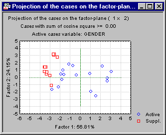
This plot shows the factor coordinates for all observations, that is, both the active observations (cases) that were used to compute the current factor solution (namely, Females) as well as the supplementary observations (cases) that are only mapped into the coordinate system defined by the two factors (Males). One interesting result that is apparent in this plot pertains to the clustering of active and supplementary cases. It appears that all supplementary cases (Males, plotted as red squares) in the analysis are plotted to the left of the center of the first axis (that is, have negative coordinate values for the first, horizontal axis). Given the interpretation of this factor as Work versus Home-related activities, with WORK and TRANSPORT defining the negative (left) side of this dimension, it appears that the daily activities of Males in this study fall mostly on the Work side of this dimension.

Summary

The purpose of this example is to illustrate how the Principal Components and Classification Analysis module can be used as a tool for first identifying important dimensions in a set of variables, then to map into those dimensions other variables of interest, and to identify clusters of observations with similar characteristics with respect to these dimensions.