Example 4: Predictive Data Mining for Categorical Output Variable (Classification)
The purpose of this example is to illustrate the power and ease of use of Statistica Data Miner projects for advanced predictive data mining (see also Crucial Concepts in Data Mining and Data Mining Tools.
Specifically, with the Workspace menu commands General Classifier (Trees and Clusters) and General Modeler and Multivariate Explorer, you can display pre-wired Statistica Data Miner projects with automatic deployment that include collections of very advanced and powerful techniques for predictive data mining. These methods can work in competition or in unison to produce averaged, voted, or best predictions (see also meta-learning).
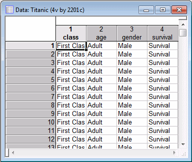
Open the Titanic.sta example data file.
This file contains information on the gender, age, type of accommodation (class), and ultimate survival status for the passengers of the ill-fated vessel.
Advanced Comprehensive Classifiers project
- Ribbon bar
- Select the
Data Mining tab. In the
Tools group, click
Workspaces, and from the
General Classifier (Trees and Clusters) submenu, select
Advanced Comprehensive Classifiers Project.
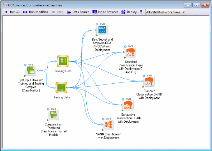
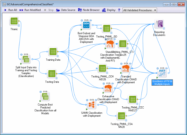
The GCAdvancedComprehensiveClassifiers.sdm project is displayed, which consists of a single entry point (node), for connecting the data and numerous nodes for fitting various models to those data.
The single connection point for the data is the Split Input Data into Training and Testing Samples (Classification) node. Using random sampling [which can be controlled in the Split Input Data into Training and Testing Samples (Classification) dialog box], this node splits the sample of observed classifications (and predictors) into two samples: one Training sample and one Testing sample (marked for deployment; see option Data for deployed project; do not re-estimate models in the Select dependent variables and predictors topic).
The models are fitted using the Training sample and evaluated using the observations in the Testing sample. By using observations that did not participate in the model fitting computations, the goodness-of-fit statistics computed for predicted values derived from the different fitted models can be used to evaluate the predictive validity (accuracy) of each model, and hence can be used to compare models and to choose one or more over others.
The Compute Best Predicted Classification from all Models node automatically computes predictions from all models by either computing a voted prediction (see voting, bagging) or choosing the best prediction, or a combination of the two (see also Meta-learning). These predictions are placed in a data spreadsheet that can be connected to other nodes (e.g., graphs) to summarize the analysis.
In summary, the Advanced Comprehensive Classifiers project applies a suite of very different methods to the classification problem and automatically generates the deployment information necessary to classify new observations using one of those methods or combinations of methods..
Specifying the analysis
To analyze the predictors of survival for the Titanic maritime disaster, click the Data Source button on the Statistica workspace toolbar.
Select the data file Titanic as the input data source.
Select the yellow diamond icon on the middle-right side of the data source node, and drag to the Split Input Data into Training and Testing Samples (Classification) node to connect them.
Double-click the data source node to display the Select dependent variables and predictors dialog box.
Click the Variables button
Select variable survival as the Dependent; categorical variable, and variables class, age, and gender as the Predictor; categorical variables.
Click OK in the variable selection dialog box.
Click OK in the Select dependent variables and predictors dialog box.
Again, in a real-world application it is absolutely essential to first perform some careful data checking either interactively or by using the nodes and options available in the Data folder of the Node Browser (see also Crucial Concepts in Data Mining and Example 1) to ensure that the data is clean, i.e., does not contain erroneous numbers, miscoded values, etc. Skip this (usually very important) step for this example, since we already know that the example data file Titanic contains verified values.
On the workspace toolbar, click Run all.
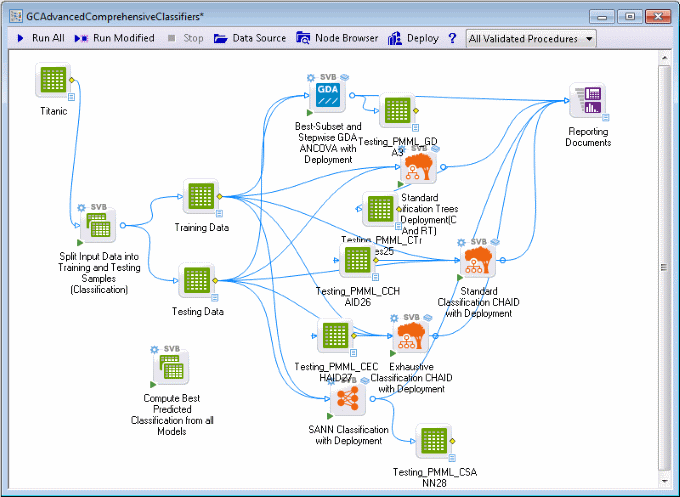
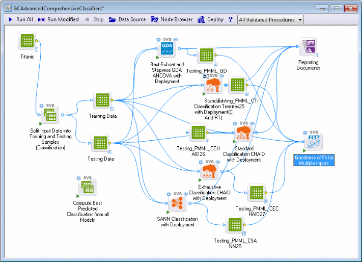
A large number of documents are produced; predicted and observed values for the observations in the testing sample, for each type of model, are placed into generated data sources labeled Testing... for subsequent analyses. Detailed results statistics and graphs for each analysis are placed into the Reporting Documents workbook. Double-click the workbook to review the results for each model.
Evaluating models
After training the system, misclassification rates are automatically computed for each node (method or model) from the testing data. This information will be used by the Compute Best Predicted... node, for example, to select the best classification method (model), or to compute the voted response for the best two or three methods (see also Meta-learning). You can review this information in the Global Dictionary, which acts as a project-wide repository of information generated by the scripts (marked ...with Deployment).
Select the Edit tab. In the Dictionary group, click Edit.
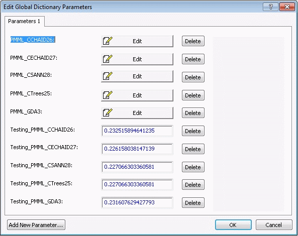
The Edit Global Dictionary Parameters dialog box is displayed, where you can review the information generated by the nodes in this project.
Even if you followed along through this example exactly step by step, the information that you see in this dialog box may differ somewhat from that displayed here because the random split of the data into training and testing sets and other method-specific random selections applied to the analyses (e.g., in neural networks) may produce slightly different results each time.
The information displayed shows for which nodes deployment information currently exists, and the misclassification rates when each of the fitted models is used to classify observations in the testing sample. Note that Testing_method_number refers to the name of the input data source, the method used to generate the prediction, and a number referring to the specific node (model) that generated the prediction (see also the description of the Show Node Identifiers option, available on the View tab). You can see that the tree classifier (CHAID) made predictions for the Testing sample, which resulted in the lowest misclassification rates.
The Goodness of Fit for Multiple Inputs node
Using the he Goodness of Fit for Multiple Inputs node is one way to evaluate the different models. This tool uses the testing output spreadsheets from each model building tool as input.
Select all of the testing output nodes: Testing_PMML_GDA, Testing_PMML_CTrees, Testing _ PMML_CCHAID, Testing_PMML_CECHAID, and Testing_PMML_CSANN.
In the Feature Finder, type good. In the list, select Goodness of Fit for Multiple Inputs (SVB).
Variable selections should be made for each of these output spreadsheets.
Double-click the GDA output spreadsheet, Testing_PMML_GDA, generated by the General Discriminate Analysis node to display the Select dependent variables and predictors dialog box.
Click the Variables button to display the variable selection dialog box.
For the Dependent, categorical variable, select survival. For the Predictor, categorical variable, select GeneralDiscriminantAnalysisPred. Click OK in the variable selection dialog box.
In the Select dependent variables and predictors dialog box, select the Always use these selections, overriding any selections the generating node may make check box. Click OK.
Repeat this process for the remaining testing output spreadsheet nodes, selecting the variable that ends with Pred for the Predictor, categorical variable.
Double-click the Goodness of Fit for Multiple Inputs node.
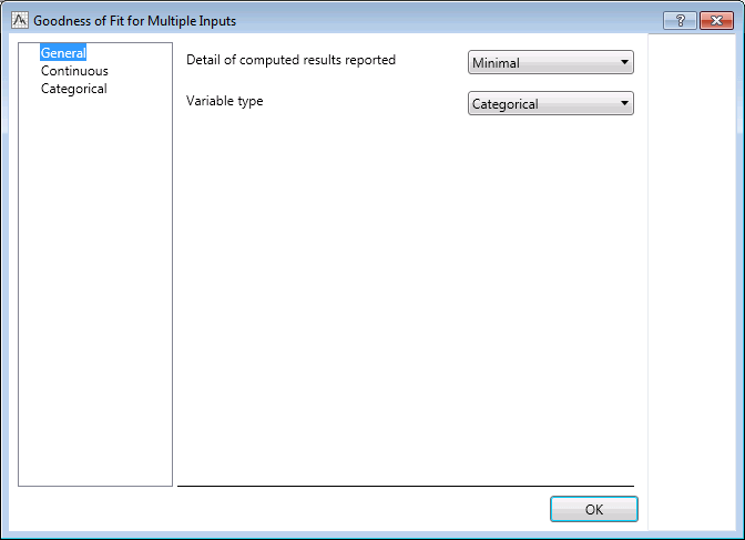
On the General tab, on the Variable type drop-down list, select Categorical.
On the Categorical tab, select the Percent disagreement check box. Click the OK button.
Run the project.
Double-click the Reporting Documents workbook to see to see the results.
The last output spreadsheet gives the overall summary of all models and all tests. Percent disagreement is lowest for the CHAID model, row 2 of the summary output, 21.5867.
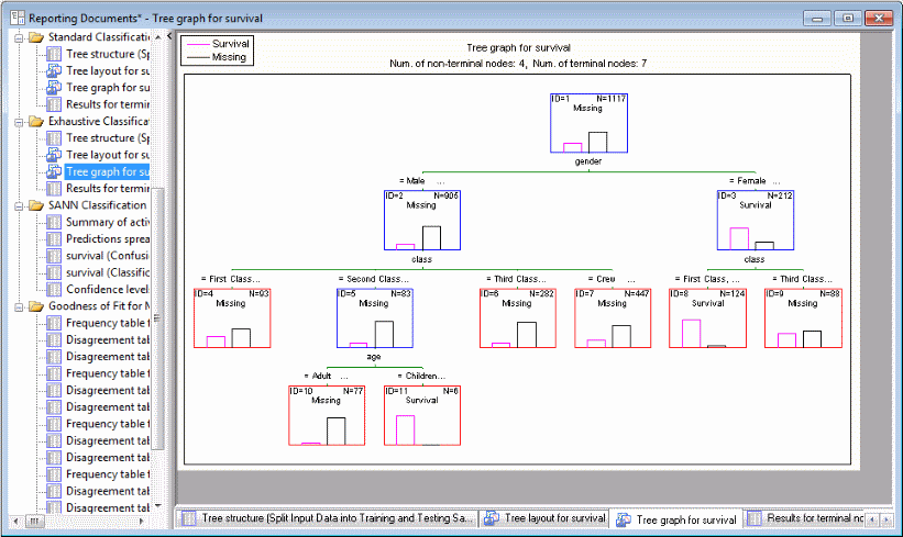
Browse through the results workbook to the Exhaustive CHAID folder to see the specific solution generated by this classifier.
If you follow this decision tree (see also Classification and Regression Trees), you will see that women in first and second class were predicted to have a much higher chance of survival, as did male children in first and second class (there were no children crew members). This solution, which could have been expected, nevertheless demonstrates that the program found a sensible model for predicting classifications.
Deployment: Computing Predicted Classifications
While deployment – predicting classifications for new cases where observed values do not exist (yet) – isn't useful in the present example, you could, nevertheless, now attach to the Compute Best Prediction from All Models node a new data source that has missing data for the categorical dependent variable (see also Example 3 for prediction of a continuous dependent variable from multiple models). The program would then compute predicted classifications based on a vote (which categories gets the most predictions) made by all models. This is the default method of combining different models used by the Compute Best Prediction... node; you can display the dialog box for that node to select one of the other methods for combining predicted classifications as well.
The Best prediction and Vote of best k predictions options would automatically identify (based on the Testing sample misclassification rates) which models were most accurate, and use those models to compute a voted prediction (see also bagging, voting, or Meta-learning).
Deploying the solution to the field
To reiterate (see also Analysis Nodes with Automatic Deployment, the deployment information is kept along with the data miner project in a Global Dictionary, which is a workspace-wide repository of parameters. This means that you could now save this Data Miner project under a different name, and then delete all analysis nodes and related information except the Compute Best Prediction from All Models node and the data source with new observations (marked for deployment). You could now simply enter values for the predictor variables, run this project (with the Compute Best Prediction from All Models node only), and thus quickly compute predicted classifications. Because Statistica Data Miner, like all analyses in Statistica , can be called from other applications, advanced applications could involve calling this project from some other (e.g., data entry) application.
Ensuring that deployment information is up to date
In general, the deployment information for the different nodes that are named ...with Deployment is stored in various forms locally along with each node, as well as globally, "visible" to other nodes in the same project. This is an important point to remember, because for Classification and Discrimination (as well as Regression Modeling and Multivariate Exploration), the node Compute Prediction from All Models will compute predictions based on all deployment information currently available in the global dictionary. Therefore, when building models for deployment using these options, ensure that all deployment information is up to date, i.e., based on models trained on the most current set of data. You can also use the Clear All Deployment Info nodes in the workspace to programmatically clear out-of-date deployment information every time the project is updated.
Predicting new observations, when observed values are not (yet) available
When connecting data for deployment (prediction or predicted classification) to the nodes for Classification and Discrimination or Regression Modeling and Multivariate Exploration, ensure that the structure of the input file for deployment is the same as that used for building the models (see also the option description for Data for deployed project; do not re-estimate models in the Select dependent variables and predictors dialog box topic). Specifically, ensure that the same numbers and types of predictor variables are specified, that a (continuous or categorical) dependent variable is specified (even if all values for that variable are missing), and that the variable names match those in the data file used to build the models (this is particularly important for the deployment of neural networks, which will rely on this information). Also, when using numeric variables with text values as categorical predictors or dependent variables, ensure that consistent coding is used throughout the Data Miner project. For additional details, refer to Using text variables or text values in data miner projects; a detailed technical discussion of this issue, and the manner in which Statistica Data Miner handles text variables and values, see Working with Text Variables and Text Values: Ensuring Consistent Coding.
Conclusion
The purpose of this example is to show how easily a large number of the most sophisticated methods for predictive data mining can be applied to data, and how sophisticated ways for combining the power of these methods for predicting new observations becomes automatically available. The techniques provided in Statistica Data Miner represent some of the most advanced techniques for predictive data mining available today.
See also, Data Mining Definition, Data Mining with Statistica Data Miner, Structure and User Interface of Statistica Data Miner, Statistica Data Miner Summary, and Getting Started with Statistica Data Miner.

