Example 1: Deriving and Examining a Sampling Plan
- Overview
- This example is based on a fictitious data set contained in the data file Pistons2.sta. However, a data file is actually not necessary for this procedure if you are only deriving a sampling plan, and are not yet analyzing data using the respective sampling plan. Suppose you are producing piston rings for a small automotive engine; the target diameter of the piston rings is 74 millimeters (mm). Now, suppose that you can estimate the standard deviation of the process (sigma) from previous quality control research as sigma (σ) = 0.01. You want to inspect the batches of piston rings that you are producing so that you can detect if the average diameter shifts from specification by more than .005 millimeters.
- Specifying the Data File
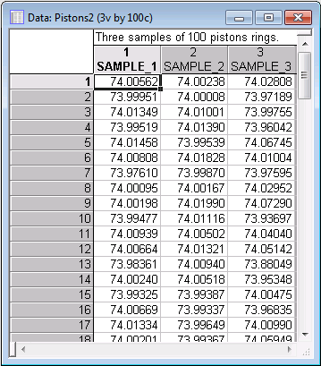
- The data in the file Pistons2.sta contains the measurements of three samples of 100 piston rings that were successively drawn by random from the production process. Open this data file.
Ribbon bar. Selecting the Home tab. In the File group, click the Open arrow and select Open Examples to display the Open a Statistica Data File dialog box. The data file is located in the Datasets folder.
Classic menus. On the File menu, select Open Examples to display the Open a Statistica Data File dialog box. The data file is located in the Datasets folder.
Variable 1 (Sample_1) was produced as a normal random variable with a mean of 74 and a sigma of .01; variable 2 (Sample_2) was produced as a normal random variable with a mean of 74.005 and a sigma of .01; variable 3 (Sample_3) was produced as a normal random variable with a mean of 74 and a sigma of .05.
- Specifying the Analysis
- Start the Process Analysis module.
- Ribbon bar
- Select the Statistics tab. In the Industrial Statistics group, click Process Analysis to display the Process Analysis Procedures Startup Panel.
- Classic menus
- On the Statistics -
Industrial Statistics & Six Sigma submenu, select
Process Analysis to display the Process Analysis Procedures Startup Panel.
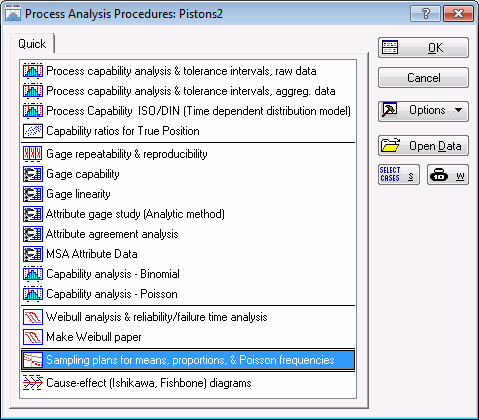
Select Sampling plans for means, proportions, & Poisson frequencies.
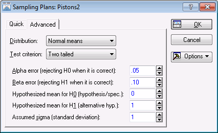
Click the OK button to display the Sampling Plans dialog box, in which you can specify the parameters that will determine the sample sizes. First, select the Advanced tab.
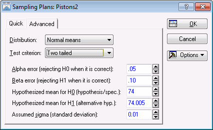
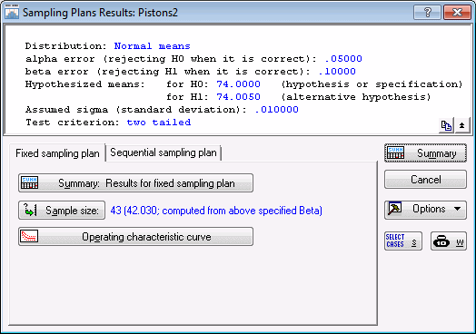
Specifying H0, H1, and the test criterion. As discussed in the Introductory Overview, in order to estimate sample sizes, you need to specify the size of the difference that you want to detect. The mean under H0 refers to the target specification; thus, enter 74 into the Hypothesized mean for H0 (hypothesis/spec) box. The mean under H1 is the one that you want to detect.
Remember that the process shift that you want to protect against is 0.005 millimeters. Because you want to detect both upward shifts of this magnitude and downward shifts, specify a Two tailed test criterion (the default) in the Test criterion list. In the case of a two-tailed test, it does not matter whether you enter as the mean under H1 74 - .005 = 73.995 or 74 + .005 = 74.005; thus, enter 74.005 as the Hypothesized mean for H1 (alternative hyp.).
If you were mostly concerned about upward shifts in the process, you would set the Test criterion box to One-sided (right) test; in that case, the mean for H1 must be greater than the mean for H0; if you were mostly concerned about downward shifts, you would set the Test criterion box to One-sided (left) test, and enter a mean for H1 that is smaller than H0.
- Specifying sigma
- As mentioned earlier, you can assume that the process standard deviation (sigma) is equal to about 0.01 mm. To specify this value, enter 0.01 in the Assumed sigma (standard deviation) box.
- Alpha/beta error
- These two parameters are discussed in the
Introductory Overview. In short, the
alpha error probability is the probability of erroneously rejecting the process, that is, declaring that a mean shift has occurred when in fact it has not.
The beta error probability is the probability of erroneously accepting the process, that is, declaring that no mean shift has occurred, when in fact it has (of the magnitude specified by the H1 mean).
The default parameters for these values are adequate, therefore, the Sampling Plans dialog box will now look like this.
- Reviewing results for fixed sampling plan
- Now, click the
OK button to display the
Sampling Plans Results dialog box.
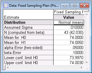
The results for a fixed sampling plan will be reviewed first. As you can see, the sample size that would be required given the previous specifications is equal to 43 (see the number beside the Sample size button). You can review the details of the fixed sampling plan in a spreadsheet by clicking the Summary: Results for fixed sampling plan button.
In addition to the previously selected specifications, the spreadsheet also shows the lower and upper confidence limits for H0. Thus, if the average piston ring size would fall below 73.997 or above 74.003 in a sample of size 43, you would say that a process shift has occurred.
- Operating characteristic (OC) curve
- After returning to the
Results dialog box, click the
Operating characteristic curve button to view the OC curve for the fixed sampling plan.
The OC curve shows the power of the fixed sampling plan (see Process Analysis Sampling Plans - Fixed Sampling Plans); that is, this plot shows how likely it is that a shift to the values indicated on the x-axis will be detected, given the current size, or for some alternative sample size.
- Specifying a sample size
- Assuming that H1 is correct, using different sample sizes in this plan will lead to different beta error probabilities (remember that the
alpha error probability is only relevant when H0 is true).
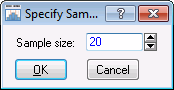
For example, try a sample size of 20. In the Results dialog box, click the Sample size button and enter 20 in the Specify Sample Size dialog box.
When you click the OK button in this dialog box, the Resultant b (beta) for that value will be displayed in the Results dialog as .39. Thus, lowering the sample size to 20 would greatly increase the likelihood that you would miss a process mean shift by .005 mm (and erroneously accept H0).
- Reviewing results for sequential sampling plan
- Now, select the
Sequential sampling plan tab. The results for an equivalent sequential sampling plan will now be reviewed. Remember that in this type of plan, you would continue to draw individual piston rings by random, and keep a running total of the sum of deviations from specification. Now, select a process that you know is in control; namely, click the
Variable containing data following current plan button to display a standard variable selection dialog box. Select variable 1 (Sample_1), and then click the
OK button.
As mentioned earlier, this variable was actually created as a random normal variable with a mean of 74 and a standard deviation of .01. However, for this example, assume that these data are actual data for 100 piston rings that you sequentially selected from the production process.
- Summary of sequential sampling plan
- Now, click the
Summary of equivalent sequential sampling plan button.
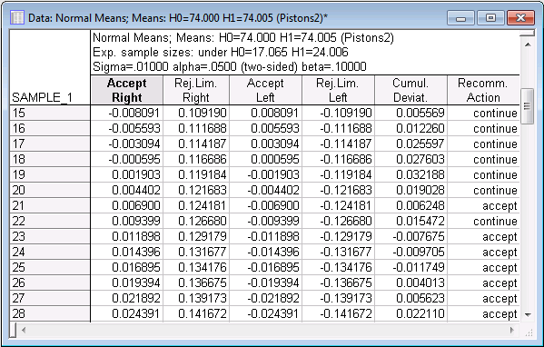
The above spreadsheet displays samples 15 through 28. As you can see, at sample 21, the Recommended Action shown in the last column is to accept the process.
Note: under the fixed sampling plan, you expected a sample size of 43 in order to arrive at this decision. In the header of the spreadsheet, you can see the expected sample sizes for the sequential plan: Given that H0 is true, you could expect an average sample size (or average run length; ARL) of 17 to 18 before arriving at an accept decision; under H1, you would expect an average sample size (ARL) of about 24 (or 25; it is always safe to round these numbers up). Thus, the sequential sampling plan is clearly more economical than the fixed plan.The spreadsheet above also shows the acceptance and rejection limits for a right- or left-shift of the process mean. These can best be visualized in a plot.
- Plot of sequential sampling plan
- After returning to the
Sequential sampling plan tab, click the
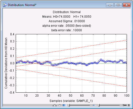
Plot equivalent sequential sampling plan button. The upper and lower rejection and acceptance limits (for right-shift and left-shift, respectively) form two "corridors."
If the cumulative sum of deviations from specification steps outside either corridor to the inside, that is, toward the center line, you accept the process as being in control. At that point you would stop sampling additional piston rings. As you already saw in the spreadsheet, this happens at around sample number 21, and you could have stopped sampling there.
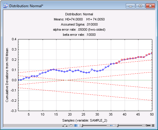
Shown below is the plot for variable 2 (Sample_2) which, as you may remember, was actually generated as a normal random variable with a mean of 74.005 and a standard deviation of .001. Assume that this sample is from a "bad" batch. Only the first 50 samples (piston rings selected from the production process) have been plotted in this chart. (To produce this plot, click the Variable containing data following current plan button and select Sample_2. Then enter 50 into the Sampling plan for sample sizes 1 through box and click the Plot equivalent sequential sampling plan button.)
As you can see, the line steps above the upper rejection limit at about sample number 37. At that point you would reject the sample and declare that the process mean has shifted by at least .005 millimeters.
- Printing empty charts for later use
- As has been mentioned earlier, you can produce sequential sampling plans without having to specify any variables, that is, before beginning to take samples (set the
Variable containing data following current plan option to
None by clicking it and then click the
Plot equivalent sequential sampling plan button).
Such empty sampling plans can be printed and then completed by hand as the engineer sequentially inspects randomly chosen units from the batch or lot.
- Summary
- To summarize, (acceptance) sampling plans make it possible for you to decide, without having to inspect 100% of the entire batch or lot, whether a mean shift of a particular size has occurred. In general, sequential plans are more economical than fixed sampling plans.
With the Process Analysis module, you can generate and analyze sampling plans for normal means (as in this example), as well as proportions (e.g., proportion of units within specification limits) and Poisson frequencies (e.g., number of defects per batch).