Special Topics Example 1 - Simultaneous Optimization of Several Response Variables in a Central Composite (Response Surface) Design

Derringer and Suich (1980) give, as an example of these procedures, the problem of finding the most desirable tire tread compound. In their example, there are four Y variables: PICO Abrasion Index, 200 percent modulus, elongation at break, and hardness. The characteristics of the product in terms of the response variables depend on the ingredients, the X variables: hydrated silica level, silane coupling level, and sulfur. The problem is to find the levels of the ingredients that produce the most desirable tire tread compound in terms of the four outcome measures.

Ribbon bar. Select the Home tab. In the File group, click the Open arrow and from the menu, select Open Examples to display the Open a Statistica Data File dialog box. Double-click the Datasets folder, and open the Tiretre.sta data set.

Classic menus. On the File menu, select Open Examples  to display the Open a Statistica Data File dialog box. The Tiretre.sta data file is located in the Datasets folder.

In the data file, as shown below, responses on the 4 dependent variables are in the first 4 columns. Levels of the 3 independent variables are in the last 3 columns and have already been recoded using the following formulas:

SILICA = ( phr silica -1.2 ) / 0.5

SILANE = ( phr silane - 50 ) / 10

SULFUR = ( phr sulfur - 2.3 ) / 0.5

Ribbon bar. Select the Statistics tab, and in the Industrial Statistics group, click DOE to display the Design & Analysis of Experiments Startup Panel.

Classic menus. On the Statistics - Industrial Statistics & Six Sigma submenu, select Experimental Design (DOE) to display the Design & Analysis of Experiments Startup Panel.

Double-click Central composite, non-factorial, surface designs to display the Design & Analysis of Central Composite (Response Surface) Experiments dialog box.

Select the Analyze design tab, and click the Variables button.

In the variable selection dialog box, select Abrasion, Modulus, Elong, and Hardness as the Dependent variables; select Silica, Silane, and Sulfur as the Indep. (factors); do not select a Blocking variable, and click OK.

The current design is a standard, three-variable, rotatable, central composite design with six center points, and standard coding of the independent variables is used (so rescaling of the independent variables is not required); thus, simply click OK to display the Analysis of a Central Composite (Response Surface) Experiment dialog box.

Derringer and Suich (1980) fitted responses on the dependent variables to a second degree polynomial, response surface model. This is the default model for standard central composite designs, i.e., the Lin/quad main eff + 2-way interactions option button is selected by default on the Model tab.

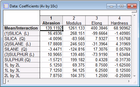
The fitted coefficients can be produced by selecting each dependent variable, in turn, from the Variable drop-down list (located at the top of the dialog box, under the Summary box), and clicking the Regression coefficients button on the ANOVA/Effects tab. The coefficients from the Regression coefficients spreadsheets for each of the four dependent variables are shown below (see also p. 218 in Derringer & Suich, 1980).

These are the regression coefficients used in computing predicted values for the dependent variables at different combinations of levels of the independent variables.

Now, to profile the predicted responses and the desirability of responses, select the Prediction & profiling tab, and click the Response Desirability Profiling button to display the Profiler.  

Response/Desirability Profiling

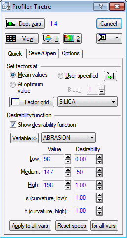
To do this, ensure that the Show desirability function check box is selected, which enables the edit fields for the Desirability function settings.

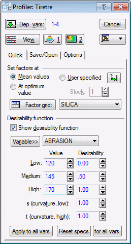
Derringer and Suich (1980) specified the desirability function for Abrasion by assigning desirability values of 0.0 (for undesirable) to predicted values of Abrasion below 120, desirability values of 1.0 (for very desirable) to predicted values of Abrasion above 170, and linearly increasing desirability values between 0.0 and 1.0 for predicted values of Abrasion between 120 and 170.

This desirability function for Abrasion is specified by entering the values of 120, 145 (the midpoint value), and 170 in the Low value, Medium value, and High value edit fields, respectively, indicating that these predicted values correspond to the three "inflection" points in the desirability function for Abrasion. The corresponding default Desirability values of 0.0, 0.5, and 1.0 are preset in the Low desirability, Medium desirability, and High desirability edit fields, respectively. Because the function does not specify any curvature in the "fall off" of desirability between inflection points, the values in the s parameter and t parameter edit fields can be left at their default values of 1.0, specifying linear changes in desirability between inflection points.

The same procedure is followed for specifying the desirability functions for the remaining three dependent variables: select the dependent variable for which to supply desirability function specifications in the Variable drop-down list, and then enter the specifications in the appropriate edit field. Derringer and Suich's (1980) specifications for the remaining three dependent variables are shown below.

A prediction profile for each dependent variable is shown, consisting of a series of graphs, one for each independent variable, of the predicted values for the dependent variable at each grid point of the independent variable, holding the levels of all other independent variables constant at their current values. By default, confidence intervals for the predicted values are also shown.

Graphs of the desirability functions for each dependent variable are displayed, and a series of graphs, one for each independent variable, shows the profile of overall response desirability at each grid point of the independent variable, holding the levels of all other independent variables constant at their current values. The overall desirability value of .17956 indicates that the mean values of the tire tread ingredients do not yield a very desirable tire tread compound, but the profile of overall response desirability also shows that a level of Sulfur lower than its mean could produce a more desirable product.

A search for the levels of the ingredients that produce the most desirable product can be conducted. This can be specified by selecting the At optimum value option button in the Set factors at group box.

To conduct the search using a general function optimization method (the simplex method), select the Options tab. Select the Use general function optimization option button in the Search options (for optimum desirability) group box.

Also, to display finer grids of predicted values and overall response desirability scores, click the Factor grid button on the Quick tab to display the Specifications for factor grid dialog box. Enter 20 for the No. of steps.  Click the accompanying Apply to all button to specify a grid of 21 points for each independent variable. Click OK to return to the Profiler.

Clicking the View button will now produce a compound response profile graph, using the optimal values of the independent variables as their current values, and 20 steps from the observed minimum to the observed maximum to define the 21 grid points for each factor.

The results displayed on the compound response profile graph show that desirability is improved by setting the factors at levels other than their means. The overall desirability value is .5833 with the settings of Silica, Silane, and Sulfur at -.0515, .1505, and -.8668, respectively. Derringer and Suich (1980) reported an overall desirability of .583 with the settings of Silica, Silane, and Sulfur at -.050, .145, and -.868, respectively, using a FORTRAN search program only briefly described in their article.

As an alternative method for conducting the search, select the Options tab. In the Search options (for optimum desirability) group box, select the Optimum desirability at exact grid points option button. Click the View button to produce a compound response profile graph, using the optimal values from the grid search as the current values for the independent variables.

The results displayed on the compound response profile graph show that the overall desirability value is .57992 with the settings of Silica, Silane, and Sulfur at 0.0, .1633, and -.8165, respectively.

With fine grids and large numbers of independent and dependent variables, the Optimum desirability at exact grid points option can take a long time to run [in this example 37,044 (or 21 x 21 x 21 x 4) predicted values and corresponding desirability scores are computed, as well 9,261 overall desirability scores], but it will always find the optimal settings for the factors.

The Use general function optimization option is generally faster, but for data sets with several local minima in overall desirability, or when the maximum desirability is close to the edge of the experimental region, the Use general function optimization search option can sometimes fail to converge or fail to find the maximum desirability (for further details on Search options, see Special Topics - Profiling Predicted Responses and Response Desirability and the Options tab on the Response/Desirability Profiler).

Surface plots and contour plots for overall response desirability are available as options in the Profiler. These plots are useful for interpreting the effects on overall response desirability of different combinations of levels of each pair of independent variables, with the remaining independent variables held constant at their current values.

Clicking the Surface button (with a number 1, located toward the top of the Profiler) will produce a compound graph with three 3-D surface plots in which pairs of independent variables are represented on two of the axes and overall response desirability is represented on the third axis.

Clicking the Contour button (with a number 2) will produce a compound graph with three contour plots showing the levels of overall response desirability produced in different regions of the plane defined by pairs of independent variables, where each region of the plane represents a different combination of the levels of the two variables.

All of these plots show that the surface is relatively flat near the maximum, meaning that small departures from the optimal settings for the independent variables would not appreciably decrease the desirability of the product. More generally, these graphic features can aid in distinguishing between factors that are "inert" and "active" with respect to other factors. For "inert" ingredients, the desirability surface or contours are "flat" with respect to an "inert" ingredient's axis. The desirability surface or contours change at different levels of an "active" ingredient.