Example 3: Variance Component Estimation for a Hierarchically Nested Random Design
- Specifying the Design
- This example illustrates variance component estimation for a hierarchically nested random effects design. Unlike full factorial designs, in which every combination of every level of each factor occurs in the design, in nested designs each level of a nested factor occurs in only one level of the factor in which it is nested. As an example, consider students who have only one classroom teacher, and teachers who teach in only one school. In a study of the variation in achievement attributable to schools, to teachers, and to students, the student factor would be nested within the teacher factor, which in turn would be nested within the school factor. The design is hierarchically nested, because there is a hierarchy of nested factors.
Example 3 is based on a fictitious data set with three independent variables A, B, and C (coded in two different ways as described below) and a single dependent variable, Y. All three factors are considered to have random effects, and Factor C is nested within Factor B, which in turn is nested within Factor A, making the design a hierarchically nested random effects design. There are unequal Ns for all three factors. The data are shown below and are available in the file Nested.sta. Open this data file via the File - Open Examples menu; it is in the Datasets folder.
As can be seen in the listing of the data set above, A1 and A2 are coded identically. B1, and C1 are coded with values identifying consecutive overall levels of the B and C nested factors, respectively, and B2 and C2 are coded with values identifying the levels within the other factors in which B and C are nested, respectively. Thus, the two sets of factors merely represent different codings of the levels of the nested factors. We will first estimate variance components for the factors in the hierarchically nested random effects design using the A1, B1, and C1 variables.
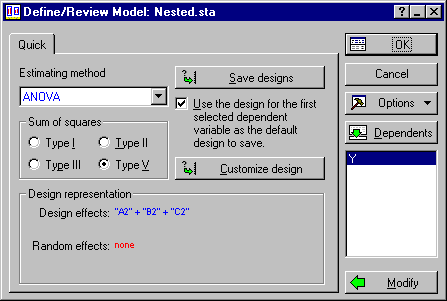
To perform the analysis, select Variance Estimation and Precision from the Statistics menu to display the Variance Estimation and Precision Startup Panel. On the Quick tab, click the Variables button to display the standard variable selection dialog. Here, select variable Y as the Dependent variable and variables A1, B1, and C1 as Grouping variables, and then click the OK button. Click OK again to display the Define/Review Model dialog. For this example we will perform an ANOVA and estimate variance components using the Type III expected mean squares method. In the Estimating method drop-down list, select ANOVA, then select the Type III option button in the Sum of squares group box.
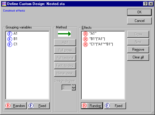
Because of the coding, STATISTICA has identified this as a nested design; however, we would like to specify different random effects. To specify a custom design, click the Customize design button to display the Define Custom Design dialog.
In the Effects pane, select A1, then click the Random button.
Click OK to return to the Define/Review Model dialog, then click OK again to display the Variance Estimation and Precision Results dialog.
- Reviewing summary results
- On the
Variance Estimation and Precision Results dialog, click the Summary button to display the Variance Estimation and Precision summary report. This report includes the Components of Variance spreadsheet, the Univariate Tests of Significance (ANOVA Results) spreadsheet, a Pareto chart for variance estimates, a variability plot, and a 2D scatterplot of predicted vs. residual values. It also provides summary information about the specified design (i.e., estimation method, dependent variables, grouping variables, and fixed/random effects). A portion of the report is shown below.
In the Report tree, click Components of Variance to display the Components of Variance spreadsheet. By default, only a portion of the spreadsheet is shown in the report. You can expand the spreadsheet by selecting it in the right pane of the report and dragging the corners of the spreadsheet.
This spreadsheet reports the variance estimates and degrees of freedom for all random effects in the model. For non-zero variance estimates, it also reports the cumulative sum of variance components, the percent of the total sum of variance components, and a relative standard deviation (RSD) that is calculated by multiplying the ratio of the variance component to the average value of all data by 100%.
To review the ANOVA results, click Univariate Tests of Significance for Y in the report tree control and, once again, expand the spreadsheet by selecting the spreadsheet object and dragging the corners.
Three graphs are also included in the Variance Estimation and Precision summary report. The Pareto chart of variance estimates indicates that the largest variance component is the Error term.
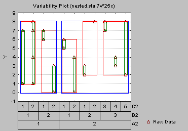
The variability plot shows the underlying organization of the data collection and is useful to evaluate the variability of one factor within several other organizing factors.
The last graph is a 2D scatterplot of predicted vs. residual values. Raw residuals are shown here; you can specify Studentized residuals on the Variance Estimation and Precision Results - Residuals tab. Additional options for residual analysis are also available on that tab.
- Specifying another analysis
- To perform the same analysis using the A2, B2, and C2 variables, click the Modify button on the
Variance Estimation and Precision Results dialog, then click the Modify button
Define/Review Model dialog to display the
Startup Panel. On the Quick tab, click the Variables button, and change the Grouping variables to A2, B2, and C2. Click the OK button on the variable selection dialog and on the Startup Panel to display the Define/Review Model dialog.
In the Estimating method drop-down list, select ANOVA, and in the Sum of squares box, select the Type III option button. In the Design representation box, notice that the suggested design is a main effect design. Recall that variables B2 and C2 are coded with values identifying the levels within the other factors in which B and C are nested, respectively. By default, Variance Estimation and Precision recognizes this as a crossed coding scheme; however, we can specify any design and Variance Estimation and Precision will analyze the data accordingly. As before, click the Customize design button to display the Define Custom Design dialog.
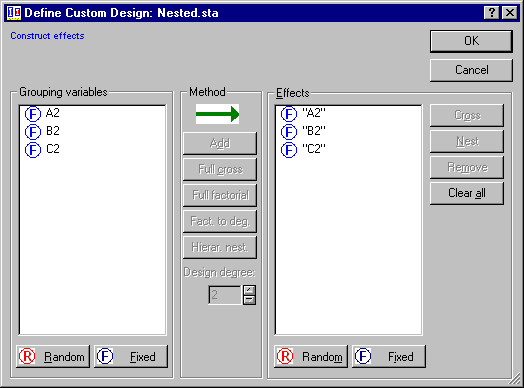
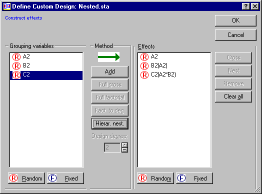
First, let's remove all the currently defined effects by clicking the Clear all button. Now, in the Grouping variables pane, select all three variables and click the Random button. Next, select A2 in the Grouping variables pane and click Add.
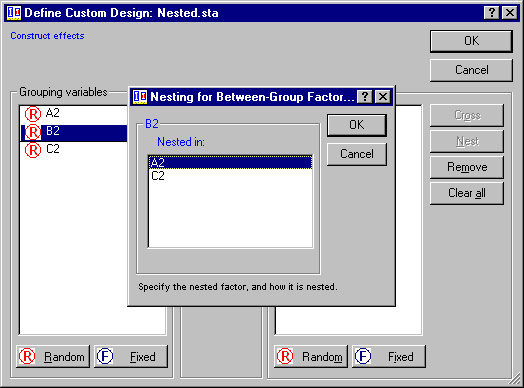
Select B2 in the Grouping variables pane, and click the Hierar. nest button to display the Nesting for Between-Group Factors dialog.
Select A2 and click OK. The random effect B2(A2) will be added to the Effects pane. Finally, select C2 in the Grouping variables pane and click the Hierar. nest button. In the Nesting for Between-Group Factors dialog, select A2 and B2 to add the random effect C2(A2*B2) to the design.
Click OK on this dialog and on the Define/Review Model dialog to display the Variance Estimation and Precision Results dialog. Once again, click the Summary button to display the Variance Estimation and Precision summary report.
You should find that the results are identical to those for the A1, B1, and C1 variables, except for the Variability Plot which reflects the "crossed" coding scheme used in variables A2, B2, and C2.
- Summary
- This example has shown how to estimate variance components for hierarchically nested random designs and how to create the Variance Estimation and Precision summary report. Two methods of coding the nested factors were illustrated. The numerical results are identical with both methods of coding, and indicate that the random factors do not significantly contribute to the variation on the dependent variable.