Example 3: Predicting Recovery from Injury
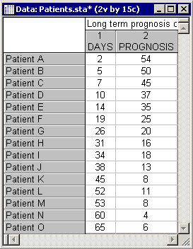
This example is also based on a data set reported in Neter, Wasserman, and Kutner (1985, page 469). Suppose a hospital administrator wants to explore the relationship between the chances for long term recovery of severely injured patients and the number of days spent in the hospital. The data file Patients.sta contains data for 15 patients; specifically, the file contains information on the number of days that each patient was hospitalized (in the variable Days) and an index of the prognosis for long-term recovery for each patient (in the variable Prognos; larger values reflect a better prognosis). Open this data file by selecting Open Examples from the File menu (classic toolbar) or by selecting Open Examples from the Open menu on the Home tab (ribbon bar); it is in the Datasets folder.
- Specifying the analysis
- Select Nonlinear Estimation from the Statistics - Advanced Linear/Nonlinear Models menu to display the Nonlinear Estimation Startup Panel. Neter et al. (1985) fit the following regression model to the data:
y = b0 * exp(b1*x)
where y denotes the prognosis and x represents the number of days that each patient was hospitalized. This model is not offered in the Nonlinear Estimation Startup Panel; therefore, you will have to double-click the User-specified regression, custom loss function option in the Startup Panel to display the User-Specified Regression, Custom Loss dialog.
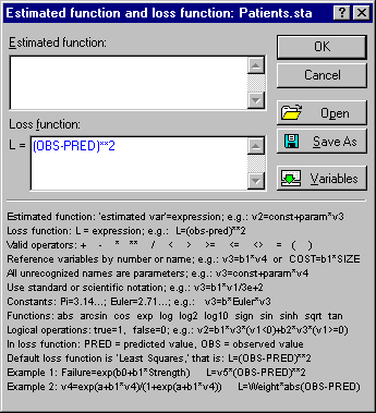
You will now need to specify the regression function. Thus, click the Function to be estimated & loss function button on the Quick tab to display the Estimated function and loss function dialog.
As you can see below, you can specify essentially any kind of model via this editor. The syntax for this dialog is reviewed in the Nonlinear Estimation - Syntax (User Functions) topic. The most important rules to remember when entering functions are:
(1) Variables can be referenced by their names or by using the convention Vxxx where xxx is the number of the variable to be referenced;
(2) All unrecognized names are interpreted as parameters to be estimated by the model.
Type in the exponential regression equation (PROGNOSIS=Param1*Exp(Param_2*DAYS)) in the Estimated function box and accept the default loss function in the Loss function box.
As you can see, the specification of regression models is rather straightforward. Note that instead of actual variable names, you could have typed in v1 and v2; also, instead of Param_1 and Param_2 to refer to the parameters, you could have used b1 and b2 or any other name that is not a valid variable name or reserved keyword.
- Loss function
- The idea of loss functions is reviewed in the Introductory Overviews. In the loss function equation, the keywords PRED and OBS refer to the predicted and observed values, respectively. Thus, the default loss function shown in the illustration above specifies the ordinary least squares estimation (predicted minus observed squared). Typically, for least-squares estimation, you should select User-specified regression, least squares from the Nonlinear Estimation Startup Panel. STATISTICA implements specific algorithms that are particularly efficient for estimating arbitrary (user-defined) regression models fitted by minimizing the least squares loss function. See also
Nonlinear Estimation Procedures - Least Squares Estimation for additional details. However, for illustration purposes, in this example we will proceed to use the more general methods that can accommodate custom loss functions as well.
Remember that complex equations can easily be saved in this dialog via the Save As button and opened for future use using the Open button. Once you click the OK button in this dialog, STATISTICA will check the syntax of the functions, and if it is acceptable it will return to the User-Specified Regression, Custom Loss dialog.
- Reviewing results
- Now, click the OK button in this dialog to display the
Model Estimation dialog.
Select the Asymptotic standard errors check box and then click the OK button to accept all the other default selections. A window is briefly displayed containing the values of the loss function and the current estimate for each parameter at each iteration. After a few iterations the estimation procedure will converge, that is, arrive at the final parameter estimates and the Results dialog is displayed.
- Reviewing the Results
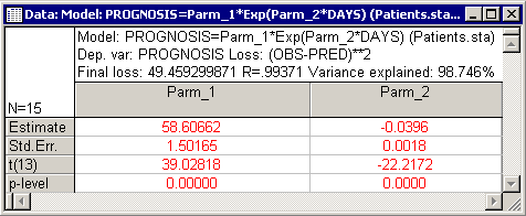
- The Results dialog shows that overall, 99% of the variability in the prognosis index from the number of days that patients are hospitalized can be explained.
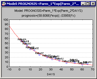
The closeness of the fit of the model to the data is also evident when you plot the fitted function; click the Fitted 2D function & observed values button on the Quick or Advanced tab to produce the graph showing the fitted function and the observed values.
The parameter estimates are shown below (click the Summary: Parameters & standard errors button).
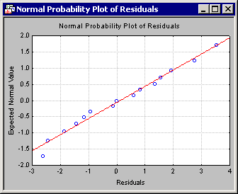
As you can see, both parameters in this model are highly significant. Click the Normal probability plot of residuals button on the Residuals tab to evaluate the adequacy of the model fit.
The residuals appear to follow closely the normal distribution; thus, it appears that the exponential model provides an adequate fit to the data.