Structural Equation Modeling and the Path Diagram
Path Diagrams play a fundamental role in structural modeling. Path diagrams are like flowcharts. They show variables interconnected with lines that are used to indicate causal flow.
One can think of a path diagram as a device for showing which variables cause changes in other variables. However, path diagrams need not be thought of strictly in this way. They may also be given a narrower, more specific interpretation.
Consider the classic linear regression equation
Y = aX + E
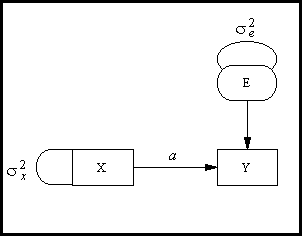
Any such equation can be represented in a path diagram as follows:

Such diagrams establish a simple isomorphism. All variables in the equation system are placed in the diagram, either in boxes or ovals. Each equation is represented on the diagram as follows: All independent variables (the variables on the right side of an equation) have arrows pointing to the dependent variable. The weighting coefficient is placed above the arrows. The above diagram shows a simple linear equation system and its path diagram representation.
Notice that, besides representing the linear equation relationships with arrows, the diagrams also contain some additional aspects. First, the variances of the independent variables, which we must know in order to test the structural relations model, are shown on the diagrams using curved lines without arrowheads attached. We refer to such lines as wires. Second, some variables are represented in ovals, others in rectangular boxes. Manifest variables are placed in boxes in the path diagram. Latent variables are placed in an oval or circle. For example, the variable E in the above diagram can be thought of as a linear regression residual when Y is predicted from X. Such a residual is not observed directly, but calculated from Y and X, so we treat it as a latent variable and place it in an oval.
The example discussed above is an extremely simple one. Generally, we are interested in testing models that are much more complicated than these. As the equation systems we examine become increasingly complicated, so do the covariance structures they imply. Ultimately, the complexity can become so bewildering that we lose sight of some very basic principles. For one thing the train of reasoning which supports testing causal models with linear structural equations testing has several weak links. The variables may be non-linear. They may be linearly related for reasons unrelated to what we commonly view as causality. The ancient adage, "correlation is not causation" remains true, even if the correlation is complex and multivariate. What causal modeling does allow us to do is examine the extent to which data fail to agree with one reasonably viable consequence of a model of causality. If the linear equations system isomorphic to the path diagram does fit the data well, it is encouraging, but hardly proof of the truth of the causal model.
Although path diagrams can be used to represent causal flow in a system of variables, they need not imply such a causal flow. Such diagrams may be viewed as simply an isomorphic representation of a linear equations system. As such, they can convey linear relationships when no causal relations are assumed. Hence, although one might interpret the diagram in the above figure to mean that "X causes Y," the diagram can also be interpreted as a visual representation of the linear regression relationship between X and Y.
