Example 12: Getting Started Constructing a D-Optimal Design
Designing the experiment. Start the Experimental Design (DOE) analysis.
Ribbon bar. Select the Statistics tab, and in the Industrial Statistics group, click DOE to display the Design & Analysis of Experiments dialog box.
Classic menus. On the Statistics - Industrial Statistics & Six Sigma submenu, select Experimental Design (DOE) to display the Design & Analysis of Experiments dialog box.
Select the Advanced tab, and select Experimental Design Builder.
Click the OK button to display the Experimental Design Builder.
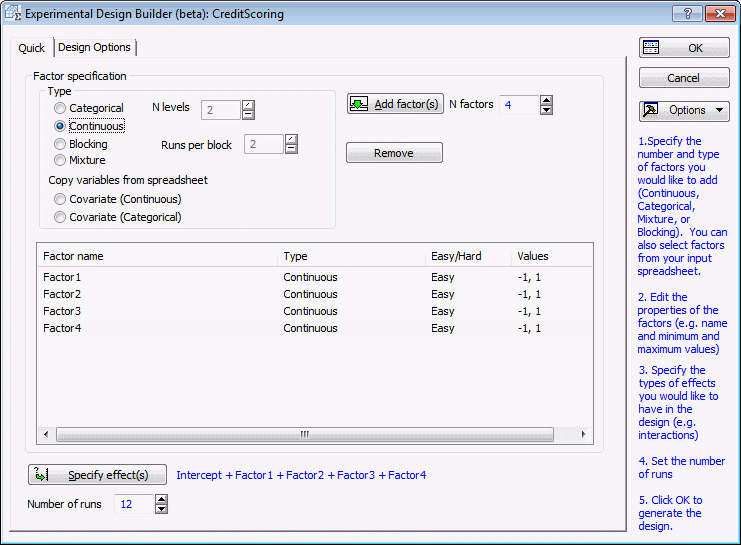
Suppose that we are interested in setting up an experiment that contains 4 continuous predictor variables: x1, x2, x3, x4. We have enough resources to perform up to 12 runs of the experiment. This number is less than the 16 runs required to perform 1 replicate of a complete factorial experiment [assuming that we only consider 2-levels (low/high) for each predictor].
Recall that D-optimal designs all will minimize the confidence ellipsoid of the estimated regression coefficients, which translates into precise estimation.
Set up the design. Set N factors to 4.
Set factor Type to Continuous.
Click the Add factor(s) button.
Set Number of runs to 12.
Click OK to generate the design and display the Experimental Design Builder Results dialog box.
On the Order of runs drop-down list, select Sort from left to right.
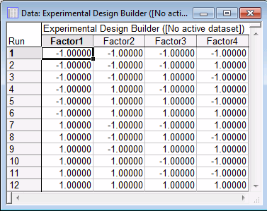
Click the Summary: Display Design button to display the design. Note that your design may look slightly different, but should be similar to the design shown below.
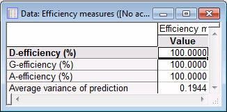
To evaluate the design, select the Design summary tab. Click the Efficiency measures button.
The D-efficiency measure compares the determinant of the current design to the determinant of an ideal orthogonal design. The determinant of the ideal orthogonal design is np. In order to interpret the measure on a per parameter basis, the D-efficiency is computed as the pth root of the ratio |XTX|/np. This measure is also a function of the scaling or coding of the predictors in the design. Due to these limitations, you should use these measures to help you decide which design to use among competing designs with an equal number of runs and where the coding or scaling of the predictors is consistent.
For this experiment, all the efficiency measures are 100%. See below for the corresponding formulas.
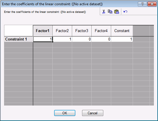
Next, let’s assume that the sum of predictors is constrained such that x1 + x2 ≤ 1. Since the current design does not account for this, we need to return to the Startup Panel and specify the constraint. Click the Cancel button in the Experimental Design Builder Results dialog box.
In the Experimental Design Builder, select the Design Options tab.
Select the Add constraints to design check box.
Click the Add constraints button.
Enter the constraints as follows.
Click the OK button.
Since we have added constraints to the design, let’s raise the Number of random starts to 1500 to increase the likelihood of a good design. Click OK to generate the design.
In the Experimental Design Builder Results dialog box, click the Summary: Display Design button to display the design. Note that your design may look slightly different, but should be similar. You can easily see that the constraint was preserved.
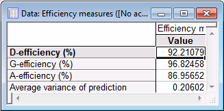
Select the Design summary tab, and click the Efficiency measures button.
The constrained design performs comparable to the unconstrained design.


