Example 14: A Multi-Trait, Multi-Method Model
When personality traits or characteristics are measured, variation among people can occur for several reasons. Two obvious contributing factors are variation in the traits themselves, and variations in the way people react to a particular method.
When a trait is measured by only one method, there is a possibility that the variation observed is actually method variance, rather than trait variance. For example, if a particular questionnaire does not control for acquiescence response set, variation among people due to a problem in the method is confounded with actual trait variation.
One way around this problem is to try to measure both trait and method variation in the same experiment. The multi-trait, multi-method correlation matrix contains correlations between t traits or characteristics each measured by the same m methods. Campbell and Fiske (1959) suggested that the multi-trait, multi-method correlation matrix should be examined to provide evidence of construct validity.
In their original work, Campbell and Fiske suggested that two kinds of validity, which they termed convergent validity and discriminant validity, could be evaluated by examining this matrix. There are 4 kinds of correlations in the matrix:
(1) same-trait, same-method
(2) same-trait, different-method
(3) different-trait, same-method
(4) different-trait, different-method.
Convergent validity is demonstrated if same-trait, different-method correlations are large. Discriminant validity is evidenced if same-trait different-method correlations are substantially higher than different-trait, different-method correlations.
Kenny (1979) analyzed data from Jaccard, Weber, and Lundmark (1975). Their study measured two traits, attitude toward cigarette smoking (C) and attitude toward capital punishment (P), with 4 different methods. The methods were:
(1) semantic differential
(2) Likert
(3) Thurstone
(4) Guilford
The correlation matrix, based on only 35 observations, is in the Jaccard.sta data file.
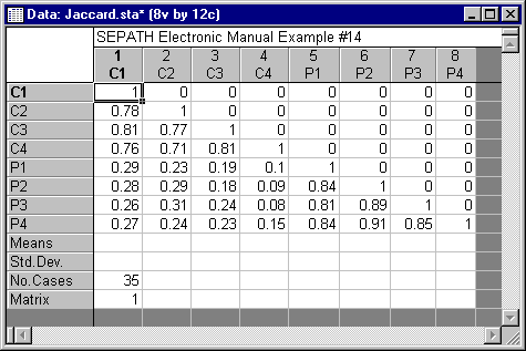
Kenny used a classic test theory approach to analyzing the data. The traits are factors whereas the disturbances or unique factors are allowed to be correlated across measures using the same method. Such a model is identified if there are at least two traits and three methods. Assuming the model fits the data, then convergent validation is assessed by high loadings on the trait factors, discriminant validation by low to moderate correlations between the trait factors, and method variance by highly correlated disturbances.
The path diagram for the resulting model is shown below. The PATH1 specification for the model is in the file Jaccard.cmd.
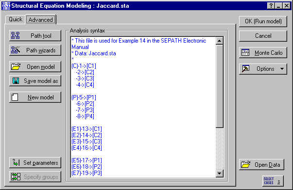
Kenny remarked that the data fit the model well in this case. With statistically-based fit indices, and the 20-20 vision of hindsight, we can see that the issue is very much in doubt. Run the example with SEPATH and see for yourself. First analyze the problem using the Analyze Covariances option (select the Covariances option button under Data to analyze on the Analysis Parameters dialog, accessed by clicking the Set parameters button on the Advanced tab of the Structural Equation Modeling (Startup Panel).
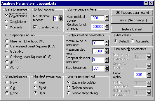
Click the OK (Accept parameters) button on the Analysis Parameters dialog to accept the options selected and return to the Startup Panel. Click the OK (Run model) button on the Startup Panel. A dialog will be displayed that says "You are analyzing a correlation matrix as if it were a covariance matrix. Results may be incorrect!" Click the OK button to display the Iteration Results dialog. Click the OK button here to display the Structural Equation Modeling Results dialog. On this dialog, click the Summary button. Examine the output, paying particular attention to the standard errors.
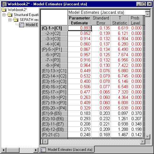
Then use the Analyze Correlations option to analyze the problem correctly (select the Correlations option button under Data to analyze on the Analysis Parameters dialog, accessed by clicking the Set parameters button on the Advanced tab of the Structural Equation Modeling (Startup Panel).
Again, after producing the output, examine the standard errors.
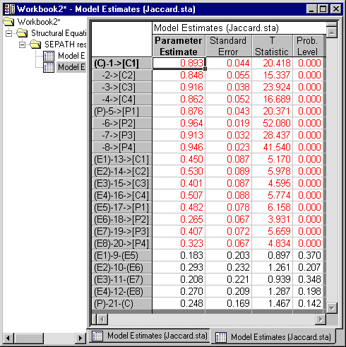
Notice how some of the standard errors differ dramatically when the sample correlation matrix is analyzed correctly.
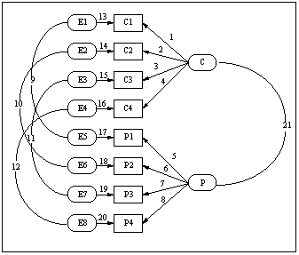
The output exhibits high loadings on the trait factors (coefficients 1 through 8), and a low correlation between the two trait factors. Disturbances are correlated, but not too highly.
The sample size is so small that the confidence intervals for the statistically-based fit indices are quite wide. For example, the 90% confidence interval for the Steiger-Lind RMS index ranges from 0 to .1056. In practice, we would prefer a substantially larger sample size.
