Example1: Canonical Correlation
This example is based on an imaginary data file Factor.sta, describing a study of life satisfaction. This data file is also analyzed in the Example section of Factor Analysis.
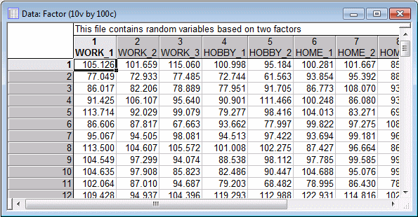
Let us assume that a questionnaire is administered to a random sample of 100 adults. The questionnaire contains 10 items that are designed to measure satisfaction at work, satisfaction with hobbies (leisure time satisfaction), satisfaction at home, and general satisfaction in other areas of life. Responses to all questions are recorded through computer, and scaled so that the mean for all items is approximately 100.The results are entered into the Factor.sta data file (see the partial listing shown below)
Procedure
- Open the Factor.sta,
-
Ribbon bar: Select the
Home tab. In the
File group, click the
Open arrow and select
Open Examples.
The Open a STATISTICA Data File dialog box is displayed.
- Open the data file, which is located in the Datasets folder.
-
Classic menus: On the
File menu, select Open Examples.
The Open a STATISTICA Data File dialog box is displayed.
-
Open the data file, which is located in the
Datasets folder.
- Purpose of analysis: Suppose that you want to learn about the relationship of work satisfaction to satisfaction in other domains. Conceptually, you will treat the work satisfaction items as the explanatory or independent variables, and the other satisfaction items as the dependent variables.
- Initial computations: Start the Canonical Analysis.
- Ribbon bar: Select the Statistics tab. In the Advanced/Multivariate group, click Mult/Exploratory and select Canonical to display the Canonical Analysis Startup Panel.
- Classic menus: To display the Canonical Analysis Startup Panel, select Canonical Analysis from the Statistics - Multivariate Exploratory Techniques menu, .
-
To display the
Select variables for canonical analysis dialog box, click the Variables button . Select all the variables, and click the
OK button.
The Startup Panel is displayed. Canonical correlation analysis is based on the correlation matrix of variables. Therefore, the first step of the analysis is to compute that correlation matrix (unless a Correlation Matrix input file is specified through the Input File drop-down list, in which case the input needs to be a correlation matrix).
- To compute the detailed descriptive statistics that is, means, correlations, covariances) for the variables in the current analysis, select the Review descriptive statistics and correlation matrix check box in order .
- To display the Review Descriptive Statistics dialog box, click the OK button.
Visualizing the Distribution of Variables
Procedure
-
Click the
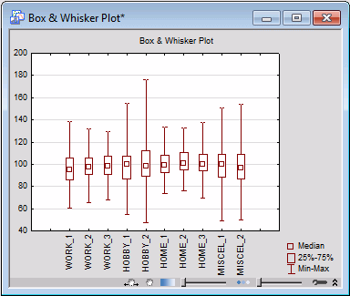
Box & whisker plot of vars button, and in the
variable selection dialog box,select all the variables. Click the
OK button.
The Box-Whisker Type dialog box is displayed, in which you can select from four types of box and whisker plots. For this example, select the Median/Quart./Range option button and then click the OK button).
Box & whisker plots are useful to determine if the distribution of a variable is symmetrical. If the distribution is not symmetrical, you may want to view the histogram for the respective variable.
- Click the Matrix plot of correlations button, and select all of the variables in the variable selection dialog. Click OK to produce a matrix of scatterplots.
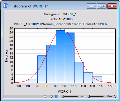
- Click the Means & standard deviations button on the Advanced tab to create a spreadsheet containing the means and standard deviations of the selected variables. As in most other modules, the default plot for the spreadsheet of means and standard deviations is the histogram of the distribution of the respective variable. This histogram will show the normal curve superimposed over the observed distribution, to provide a visual check for any violations of the normality assumption.
Specifying the Canonical Analysis and Variables
Procedure
- Click the OK button to exit the Review Descriptive Statistics dialog box and display the Model Definition dialog box, in which you can select the left and right set variables.
To specify variables for the two sets:
- Click the Variables for canonical analysis button on the Quick tab to open a standard variable selection dialog box. Select the work satisfaction variables, for example variables Work_1, Work_2, and Work_3 in the First variable list, and the remaining satisfaction items such as variables Hobby_1, Hobby_2, Home_1, Home_2, Home_3, Miscel_1, Miscel_2 in the Second variable list.
-
Click the
OK button.
Note: The designation of first and second list is arbitrary here; that is, you could also select the work satisfaction items into the second list and the remaining satisfaction items into the first list. In a sense, Canonical Analysis is completely "symmetrical," that is, it will compute the same statistics (loadings, weights, etc.) for the variables in both lists.
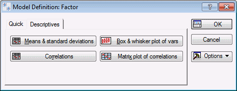
You can also use some other options, such as the Means & standard deviations or Correlations buttons, as well as create some useful descriptive graphs via the Descriptives tab.
Reviewing results: After specifying the two lists of variables, you can begin the analysis.
- Click the OK button in the Model Definition dialog box to display the Canonical Analysis Results dialog box.
The nature of most of the statistics reported here in the results summary are reviewed in the Introductory Overview section of this module. Therefore, the focus in this example will be on the interpretation of the results.
-
Click the
Summary: Canonical results button on the
Quick tab or the
Canonical factors tab to create the Canonical Analysis Summary spreadsheet.
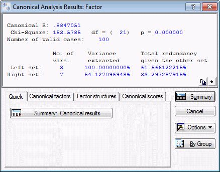
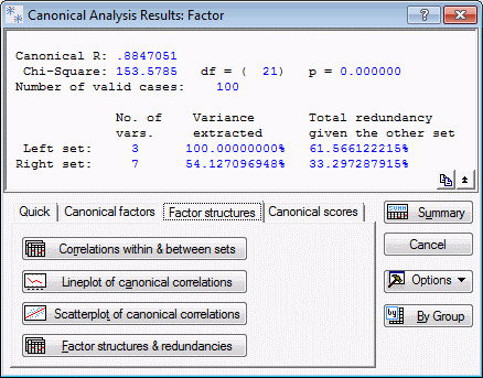
Canonical R: The overall canonical R is fairly substantial (.88), and highly significant (p< .001). Remember that the canonical R reported here pertains to the first and most significant canonical root. Thus, this value can be interpreted as the simple correlation between the weighted sum scores in each set, with the weights pertaining to the first (and most significant) canonical root.
Overall Redundancy: The values in the rows labeled Variance extracted and Total redundancy give an indication of the magnitude of the overall correlations between the two sets of variables, relative to the variance of the variables. This is different from the canonical R-square, because the latter statistic expresses the proportion of variance accounted for in the canonical variates (see the Introductory Overview for further details).
Variance extracted: The values in the Variance extracted row indicate the average amount of variance extracted from the variables in the respective set by all canonical roots. Thus, all three roots extract 100% of the variance from the left set, that is, the three work satisfaction items, and 54% of the variance in the right set. Note that one of these values will always be 100% because STATISTICA extracts as many roots as the minimum number of variables in either set. Thus, for one set of variables, there are as many independent sums (canonical variates) as there are variables. Intuitively, it should be clear that, for example, three independent sum scores derived from three variables will explain 100% of all variability.
Redundancy: The computation of the Total redundancy is explained in the Introductory Overview section. These values can be interpreted such that, based on all canonical roots, given the right set of variables (the seven non-work related satisfaction items), you can account for, on the average, 61.6% of the variance in the variables in the left set (the satisfaction items). Likewise, you can account for 33.3% of the variance in the non-work related satisfaction items, given the work related satisfaction items. These results suggest a fairly strong overall relationship between the items in the two sets.
Testing the significance of Canonical roots: Now, check whether all three canonical roots are significant. Keep in mind that the canonical R reported in this spreadsheet represents only the first root, that is, the strongest and most significant canonical correlation.
To test the significance of all canonical roots
-
Click the
Chi square tests button on the
Canonical factors tab of the
Canonical Analysis Results dialog box. The results are displayed in Chi-Square with Successive Roots Removed spreadsheet.
The maximum number of roots that can be extracted is equal to the smallest number of variables in either set. Since three work satisfaction items were selected into the first set, STATISTICA would be expected to extract three canonical roots.
The sequential significance test works as follows. First, look at all three canonical variables together, that is, without any roots removed. That test is highly significant. Next, the first (and, as you know, most significant) root is "removed" and the statistical significance of the remaining two roots is determined. That test (in the second row of the spreadsheet) is not significant. You can stop at this point and conclude that only the first canonical root is statistically significant, and it should be examine further. If the second test were also statistically significant, you would then proceed to the third line of the spreadsheet to see whether the remaining third canonical root is also significant.
Factor structure and redundancy: You now know that you should consider further only the first canonical root. How can this root be interpreted, that is, how is it correlated with the variables in the two sets? As discussed in the Introductory Overview, the interpretation of canonical "factors" follows a similar logic to that in Factor Analysis. Specifically, you can compute the correlations between the items in each set with the respective canonical root or variable (remember that the canonical variable in each set is "created" as the weighted sum of the variables). Those correlations are also called canonical factor loadings or structure coefficients.
You can compute those values (as well as the variance extracted for each set) through the Factor structures tab.
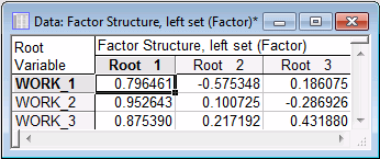
Factor structure in the left set. First, examine the loadings for the left set.
-
Click the
Factor structures & redundancies button to generate four results spreadsheets:
- Factor Structure, left set
- Variance Extracted (Proportions), left set
- Factor Structure, right set
- Variance Extracted (Proportions), rght set
Factor structure in the left set: First, examine the loadings for the left set.
Remember that only the first canonical root is statistically significant, and it is the only one that should be interpreted. As you can see, the three work satisfaction items show substantial loadings on the first canonical factor, that is, they correlate highly with that factor.
As a measure of redundancy, the average amount of variance accounted for in each item by the first root could be computed. To do so, you could sum up the squared canonical factor loadings and divide them by 3 (the number of variables in this set).
Now, look at the Variance Extracted (Proportions), left set results spreadsheet.
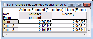
As you can see in this spreadsheet, the first canonical root extracts an average of about 77% of the variance from the work satisfaction items. If you multiply that value with the proportion of shared variance between the canonical variates in the two sets (i.e., with R-square), then the number in the Reddncy column of the spreadsheet (i.e., redundancy) is obtained. Thus, given the variables in the right set (the non-work related satisfaction items), you can account for about 60% of the variance in the work related satisfaction items, based on the first canonical root.
Factor structure in right set: In the Factor Structure, right set spreadsheet, the first canonical root or factor is marked by high loadings on the leisure satisfaction items (Hobby_1 and Hobby_2).

The loadings are much lower for the home-related satisfaction items. Therefore, you can conclude that the significant canonical correlation between the variables in the two sets (based on the first root) is probably the result of a relationship between work satisfaction, and leisure time and general satisfaction. If you consider work satisfaction as the explanatory variable, you could say that work satisfaction affects leisure time and general satisfaction, but not (or much less so) satisfaction with home life.
The Variance Extracted (Proportions), right set spreadsheet shows the redundancies for the right set of variables.
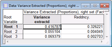
As you can see, the first canonical root accounts for an average of roughly 42% of variance in the variables in the right set; given the work satisfaction items, you can account for about 33% of the variance in the other satisfaction items, based on the first canonical root. Note that these numbers are "pulled down" by the relative lack of correlations between this canonical variate and the home satisfaction items.
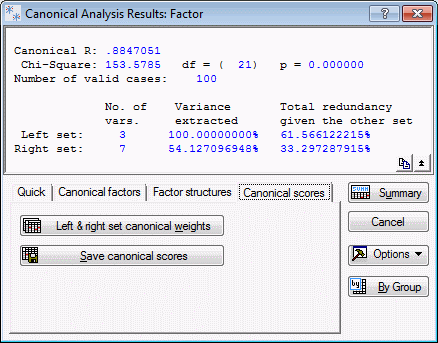
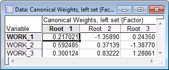
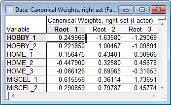
Canonical scores: Remember that the canonical variates represent weighted sums of the variables in each set. You can review those weights through the Canonical Scores tab.
-
Click the
Left & right set canonical weights button to produce two spreadsheets.
The weights shown in the Canonical Weights spreadsheets pertain to the standardized (z-transformed) variables in the two sets. You can use those weights to compute scores for the canonical variates. The scores computed from the data in the current data file may be saved via the Save canonical scores button.
Plotting canonical scores: Now, plot the canonical scores for the variables in the left set against the scores for the variables in the right set.
- On the Factor structures tab, click the Scatterplot of canonical correlations button to display the Scatterplot of Canonical Correlations dialog box. To produce a scatterplot for the first (and only significant) canonical variate, select Root 1 in the Left set box and Root 1 in the Right set box.
-
Click the
OK button to produce the scatterplot.
Note: In the illustration shown below, a linear regression line was added to the plot through the Plot: Fitting tab of Graph Options dialog box.
There are no outliers apparent in this plot, nor do the residuals around the regression line indicate any non-linear trend (e.g., by forming a U or S around the regression line). Therefore, you can be satisfied that no major violations of a main assumption of canonical correlation analysis are evident.
Clusters of cases: Another interesting aspect of this plot is whether or not there is any evidence of clustering of cases. Such clustering may happen if the sample is somehow heterogeneous in nature. For example, suppose respondents from two very different industries who are working under very different conditions were included in the sample. It is conceivable that the canonical correlation represented by the plot above could then be the result of the fact that one group of respondents is generally more satisfied with their work and leisure time (and life in general). If so, this would be reflected in this plot by two distinct clusters of points: one at the low ends of both axes and one at the high ends. However, in this example, there is no evidence of any natural grouping of this kind, and therefore you do not have to be concerned.
Conclusion: It can be concluded from the analysis of this (fictitious) data set that satisfaction at work affects leisure time satisfaction and general satisfaction. Satisfaction with home life did not seem to be affected. In practice, before generalizing these conclusions, you should replicate the study. Specifically, you should ensure that the canonical factor structure that led to the interpretation of the first canonical root is reliable (i.e., replicable).

