SANN Example 3: Growth in Number of Airline Passengers over Time
This example concentrates on a typical regression time series problem.
Data
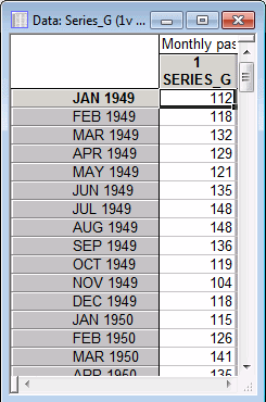
This example uses the Series_G.sta data file. The data are monthly passenger totals (measured in thousands) in international air travel, for twelve consecutive years: 1949-1960. Part of the Series_G.sta data file is as follows.
The first thing you will notice is that the data set includes only a single variable. We are using this both as the input and output of the neural network (but, of course, at different time steps). In Statistica Automated Neural Networks (SANN), a variable is considered as both input and target; no corresponding input is selected.
This example explains typical regression time series problem.

Specifying the analysis
Open the Series_G.sta data file and start SANN using one of the following ways:
- Ribbon bar. Select the Home tab. In the File group, click the Open arrow and select Open Examples to display the Open a Statistica Data File dialog box. Open the data file, which is located in the Datasets folder. Then, select the Statistics tab. In the Advanced/Multivariate group, click Neural Nets to display the SANN - New Analysis/Deployment Startup Panel. Or, select the Data Mining tab. In the Learning group, click Neural Networks to display the SANN - New Analysis/Deployment Startup Panel.
- Classic menus. From the File menu, select Open Examples to display the Open a Statistica Data File dialog box. Open the data file, which is located in the Datasets folder. Then, from the Statistics menu or the Data Mining menu, select Automated Neural Networks to display the SANN - New Analysis/Deployment Startup Panel.
- In the New analysis list box, select Time series (regression).
- Click the OK button to display the SANN - Data selection dialog box.
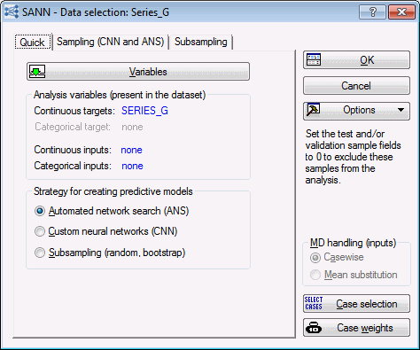
- On the Quick tab, click the Variables button. A standard variable selection dialog box is displayed, where you specify the variables for the analysis.
- You can use the variable SERIES_G as both the target and input for our neural network. To do this, you can specify the variable once, as a continuous target, while no inputs are selected.
- Select SERIES_G in the Continuous targets column, and then click the OK button. The variable selection dialog box closes, and you return to the SANN - Data selection dialog box.
- In the Strategy for creating predictive models group box, there are three strategies available for time series (regression): Automated network search (ANS), Custom neural networks (CNN), and Subsampling (random, bootstrap). Select ANS.
- Select the Sampling (CNN and ANS) tab.
Note on sampling
As with other analysis types in SANN, you are able to divide the data set into sub samples that can be used for training the data, testing the networks during training and validating the networks after training is complete. You can let SANN create these subsets (using the Random option) or you can assign cases to subsets yourself, using a sample identifier variable (Sampling variable option).
Given the nature of time series data (that is, the data represent a sequence of measurements taken at successive points in time), you might wonder how the data can be partitioned into subsets without disrupting the very time pattern that we seek to model. SANN does not actually rearrange the data into subsets. Instead, the cases are left in the current order so that the time series pattern can be identified. Splitting the data into their respective subsets occurs after the predictions have been made.
For example, consider a very short data set with 5 cases that have been randomly assigned to subsets as shown:
Case 1 - Train
Case 2 - Train
Case 3 - Test
Case 4 - Train
Case 5 - Test
In time series analyses with, for example, lag 1, the actual time series data set that is used to train and test the neural network model has two cases for training and two cases for testing. Since Case 1 has no prior entries, it has no input and therefore cannot be used at all. However, Case 1 serves as an input to Case 2, which plays the role of a target. This forms the first training case in the training sample, which consists of {Case 1, Case 2} as an input-target pair. Similarly, Case 2 is used as an input to Case 3, and the result is {Case2, Case 3}, which is used for testing, and so on.
- For this example, let’s leave the default settings as they are.
- Now, select the Time series tab.
- For time series problems, you need to make an additional design decision - the number of time series steps to use as input to the network. For some problems, determining the correct number of input steps can require a certain amount of trial-and-error. However, if the problem contains a natural cycle period (example, the Series_G.sta data file contains monthly sales figures, so there is a definite length – 12-month period – in the data), you should try specifying that cycle or an integral multiple of it.
-
In this case, we can specify a period of 12, as this is the natural cycle of the time series. To do this, enter a 12 in the Number of time steps used as inputs field.
Training the networks
- To display SANN - Automated Network Search (ANS) dialog box, click the OK button in the SANN - Data Selection dialog box .
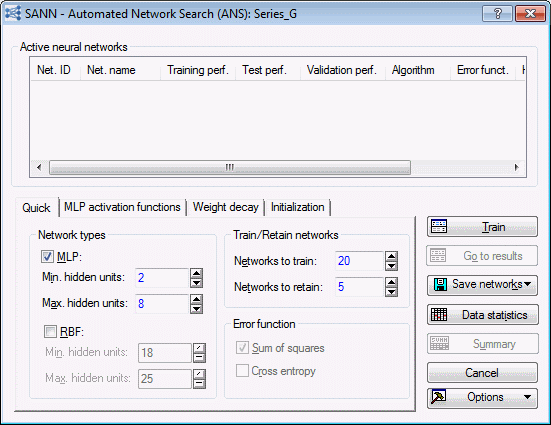
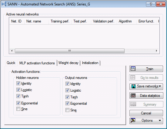
- This dialog box contains the same tabs that are available during regression analysis (Quick, MLP activation functions, Weight decay, and Initialization).
- You can configure the options on these tabs according to the needs of your experiment. For example, if you have prior knowledge that MLP neural networks are best suited for modeling your data, it is reasonable to exclude RBF networks for the analysis. You can do so by clearing the
RBF check box in the
Network types group box of the
Quick tab. Similarly, if you have reason to believe that the search range for network complexity should be widened, you can use the
Min. hidden units and
Max. hidden units options to satisfy this requirement. Alternatively, if you want to specify the network complexity, you can do so by setting Min. hidden units = Max hidden units. Note that the
Cross entropy check box is not available (in the Error function group box) since this type of error is used only in classification problems.
Note: The more networks you create, the more chance you have for finding the best solution. Usually 20 or so networks are sufficient, but this may depend on the nature of the problem at hand. You can also change the number of networks to retain, but usually retaining 5 of the best networks is sufficient. In the Results dialog box, you can use these networks to form ensembles.
- Since in most analyses the nature of the input-target relationship is often not well understood, it is advisable that you use as many activation function types as possible. This helps the ANS search for the best network activation function more thoroughly.
Reviewing the results
- In the SANN - Automated Network Search (ANS) dialog box, click the Train button.
- SANN trains and retains 5 networks. When training is complete, the SANN - Results dialog box is displayed.
- Select the Time Series tab.
- With the options on this tab, you can review a multiple scatterplot of the target (Series_G) vs. the predictions for the five models, and you can generate time series projections. You can also view the time series data the way they are presented to the network.
Review of time series predictions.
The time series predictions graph is a line graph that relates the target to the outputs (predictions of the network). When a network has closely modeled the existing data, we expect to find a strong linear relationship between the target and output of the network. When this plot results in a line nowhere close to the target values, it indicates that the networks have not adequately captured the pattern in the target. If this happens, you should try to specify a different Number of time steps used as inputs on the Time series tab of the SANN - Data Selection dialog box.
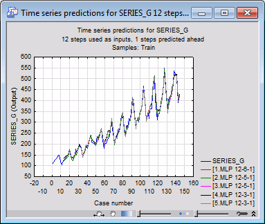
On the Time series tab, click the Time series graph button to create a line plot for the predictions of the networks against the time steps.
You can use this graph to visually verify how well the networks predict the time series data. The degree of fit is well, which again is an indication of the time series dependency in the data. Thus, for this example, all the networks seem to model the data reasonably well. Note that the first 12 cases of the graph have no predictions. That is because the number of lags used as inputs was 12.
Time series projections. When the target is projected into itself (that is, there are no inputs) SANN also provides options for making time series projections. In SANN, neural networks for time series problems perform one-step-ahead prediction - they predict the next time step from a series of previous time steps. By dropping the oldest of the original input points, adding the newly predicted value, and rerunning the network, a prediction can be made a further step ahead. This process can be repeated to generate an entire time series of predictions. Note that this functionality is not available when one or more inputs are selected.
The options in the Projection group box enable you to generate a graph or spreadsheet showing the results of projecting ahead a given number of time steps. SANN can start the time series projection either from a pattern extracted from the current data set or from a user-specified pattern. We can use the default, which is to start at the first available pattern in the data set (so we are able to compare the prediction with the entire data set).
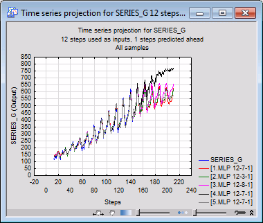
As with any prediction, errors rapidly accumulate, and such multiple-step projections can only be trusted if the network has very high predictive accuracy. Still, you should not attempt to make too many projections ahead since the predictive accuracy of the network rapidly decreases with the projection length.
The only parameters we need to set are the Projection length and Case (starts from). Our time series has only 144 cases, of which 12 are effectively removed by pre-processing (predictions cannot be made for the first twelve points, as they do not have sufficient preceding points to make the prediction), so the maximum available data to compare with is 132 steps. However, it is quite permissible to project beyond the end of the available data: you can see the predicted value projected beyond the end of the data set, although you cannot have a standard of comparison beyond that point.
As an example, you can create a projection graph with length 200 starting from case 12 by setting the value of the Projection length and Case (starts from) to 200 and 12 respectively. Then, click the Projection graph button.
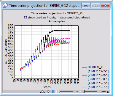
Set the projection length to 300 and create another graph by clicking the Projection graph button.
The results may seem somewhat disappointing. The prediction saturates after a time. In any event, it might actually be considered irrelevant to predict too far ahead - figures for the next year or two may be quite adequate, or the reliability of more distant predictions may be questionable. Nonetheless, this example does demonstrate a restriction of neural networks if they are blindly applied in circumstances where they are required to extrapolate beyond known data.

