k-Nearest Neighbors Introductory Overview
Classification
To demonstrate a k-nearest neighbor (KNN) analysis, let's consider the task of classifying a new object (query point) among a number of known examples. This is shown in the figure below, which depicts the examples (instances) with the plus and minus signs and the query point with a red circle. Our task is to estimate (classify) the outcome of the query point based on a selected number of its nearest neighbors. In other words, we want to know whether the query point can be classified as a plus or a minus sign.
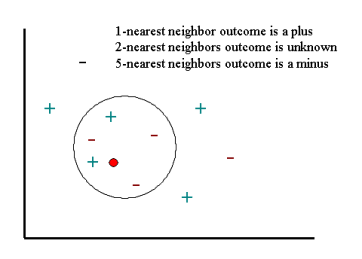
To proceed, let's consider the outcome of KNN based on 1-nearest neighbor. It is clear that in this case KNN will predict the outcome of the query point with a plus (since the closest point carries a plus sign). Now let's increase the number of nearest neighbors to 2, i.e., 2-nearest neighbors. This time KNN will not be able to classify the outcome of the query point since the second closest point is a minus, and so both the plus and the minus signs achieve the same score (i.e., win the same number of votes). For the next step, let's increase the number of nearest neighbors to 5 (5-nearest neighbors). This will define a nearest neighbor region, which is indicated by the circle shown in the figure above. Since there are 2 and 3 plus and minus signs, respectively, in this circle KNN will assign a minus sign to the outcome of the query point.
Continuous Data (Regression Problems)
In this section, we will generalize the concept of k-nearest neighbors (KNN) that has continuous dependent variables to include regression problems. The following plot represents a set of points that are drawn from the relationship between the independent variable X and dependent variable Y.
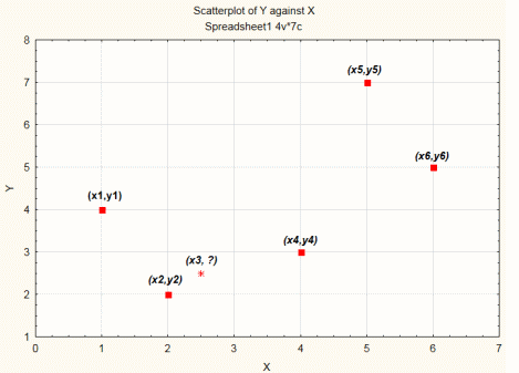
To begin with, before running the regression analysis, let's consider the 1-nearest method as an example to impute the missing value Y3. In this case, the Y3 (i.e., "?" on the plot) is obtained by locating the data points closest to (x3,?). Thus, for 1-nearest neighbor, for missing value Y3, we can write:
Y3 = y2
For the next step, let's consider the 2-nearest neighbor method. In this case, we locate the first two closest points to Y3, which happen to be (x2,y2) and (x4,y4). Thus, the missing value Y3 is given by:
Y3 = (y2 + y4)/2
This discussion can be extended to an arbitrary number of nearest neighbors k. To summarize, in a k-nearest neighbor method, the imputation for the missing value of a continuous variable is taken to be the average of its k-nearest neighbors.
Technical Details
STATISTICA k-Nearest Neighbors (KNN) is a memory-based model defined by a set of objects known as examples (also known as instances) for which the outcome are known (i.e., the examples are labeled). Each example consists of a data case having a set of independent values labeled by a set of dependent outcomes. The independent and dependent variables can be either continuous or categorical. For continuous dependent variables, the task is regression; otherwise it is a classification. Thus, STATISTICA KNN can handle both regression and classification tasks.
Given a new case of dependent values (query point), we would like to estimate the outcome based on the KNN examples. STATISTICA KNN achieves this by finding K examples that are closest in distance to the query point, hence, the name k-Nearest Neighbors. For regression problems, KNN predictions are based on averaging the outcomes of the K nearest neighbors; for classification problems, a majority of voting is used.
The choice of K is essential in building the KNN model. In fact, k can be regarded as one of the most important factors of the model that can strongly influence the quality of predictions. One appropriate way to look at the number of nearest neighbors k is to think of it as a smoothing parameter. For any given problem, a small value of k will lead to a large variance in predictions. Alternatively, setting k to a large value may lead to a large model bias. Thus, k should be set to a value large enough to minimize the probability of misclassification and small enough (with respect to the number of cases in the example sample) so that the K nearest points are close enough to the query point. Thus, like any smoothing parameter, there is an optimal value for k that achieves the right trade off between the bias and the variance of the model. STATISTICA KNN can provide an estimate of K using an algorithm known as cross-validation (Bishop, 1995).
Cross-Validation
Cross-validation is a well established technique that can be used to obtain estimates of model parameters that are unknown. Here we discuss the applicability of this technique to estimating k.
The general idea of this method is to divide the data sample into a number of v folds (randomly drawn, disjointed sub-samples or segments). For a fixed value of k, we apply the KNN model to make predictions on the vth segment (i.e., use the v-1 segments as the examples) and evaluate the error. The most common choice for this error for regression is sum-of-squared and for classification it is most conveniently defined as the accuracy (the percentage of correctly classified cases). This process is then successively applied to all possible choices of v. At the end of the v folds (cycles), the computed errors are averaged to yield a measure of the stability of the model (how well the model predicts query points). The above steps are then repeated for various k and the value achieving the lowest error (or the highest classification accuracy) is then selected as the optimal value for k (optimal in a cross-validation sense). Note that cross-validation is computationally expensive and you should be prepared to let the algorithm run for some time especially when the size of the examples sample is large. Alternatively, you can specify k. This may be a reasonable course of action should you have an idea of which value k may take (i.e., from previous KNN analyses you may have conducted on similar data) .
Distance Metric
As mentioned before, given a query point, KNN makes predictions based on the outcome of the K neighbors closest to that point. Therefore, to make predictions with KNN, we need to define a metric for measuring the distance between the query point and cases from the examples sample. One of the most popular choices to measure this distance is known as Euclidean. Other measures include Euclidean squared, City-block, and Chebyshev:
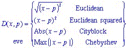
where x and p are the query point and a case from the examples sample, respectively.
K-Nearest Neighbor Predictions
After selecting the value of k, you can make predictions based on the KNN examples. For regression, KNN predictions is the average of the k-nearest neighbors outcome.
where yi is the ith case of the examples sample and y is the prediction (outcome) of the query point. In contrast to regression, in classification problems, KNN predictions are based on a voting scheme in which the winner is used to label the query.
Note. For binary classification tasks, odd values of y = 1,3,5 are used to avoid ties, i.e., two classes labels achieving the same score.
So far we have discussed KNN analysis without paying any attention to the relative distance of the K nearest examples to the query point. In other words, we let the K neighbors have equal influence on predictions irrespective of their relative distance from the query point. An alternative approach (Shepard 1968) is to use arbitrarily large values of K (if not the entire prototype sample) with more importance given to cases closest to the query point. This is achieved using so-called distance weighting.
Distance Weighting
Since KNN predictions are based on the intuitive assumption that objects close in distance are potentially similar, it makes good sense to discriminate between the K nearest neighbors when making predictions, i.e., let the closest points among the K nearest neighbors have more say in affecting the outcome of the query point. This can be achieved by introducing a set of weights W, one for each nearest neighbor, defined by the relative closeness of each neighbor with respect to the query point. Thus:
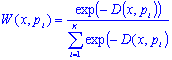
where D(x, pi ) is the distance between the query point x and the ith case pi of the example sample. It is clear that the weights defined in this manner above will satisfy:
Thus, for regression problems, we have:
For classification problems, the maximum of the above equation is taken for each class variables.
It is clear from the above discussion that when k>1, one can naturally define the standard deviation for predictions in regression tasks using: