Example 10: Capability Analysis (Binomial)
This example is based on the data also used in QC Charts Example 5: Specifying Control Charts for Attributes, Custom Control Limits. Let's assume that we are manufacturing light bulbs. To evaluate whether the individual light bulbs will operate under different conditions, we drew several samples. Each sample contained 100 bulbs. Then we performed a stress test and recorded the number of defectives (non-conforming units) in a variable Defect. At most, we will accept 10 failures out of 100 bulbs (i.e., per sample). The goal is to estimate the quality of our process (estimate process capability), for this process.
Start by opening the data file Bulbs.sta. Then, from the Statistics menu, select Industrial Statistics & Six Sigma - Process Analysis to display the Process Analysis Procedures Startup Panel.
On the Quick tab, select Capability analysis - Binomial, and click the OK button. We choose the binomial distribution for this case because the defects are independent defect counts from fixed samples of bulbs; further, each bulb has an a-priori equal probability of failing.
On the Capability analysis (Binomial) dialog - Quick tab, click the Variables button. In the variable selection dialog, select Defects in the first column as the variable with counts, and click the OK button.
Set the Sample size to 100, and enter a Target of 5 and a USL (upper specification limit) of 8. In other words, we want to target our process to yield 5 defects per 100 bulbs, with an upper specification (acceptable) limit of 8 defects per 100 bulbs.

Now, click OK to close this dialog and display the Capability analysis (Binomial) results dialog.
Observed Capability Summary
First, click the Observed Capability Summary button to review the summary of charts.
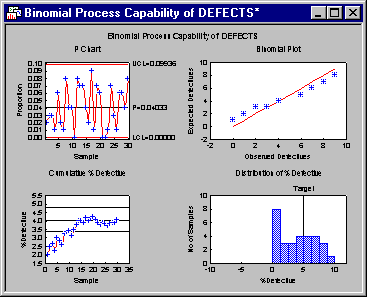
The p chart shows no samples out-of-control, so overall it appears the process is in control. The Binomial plot shows a close fit of the binomial expected frequencies to the observed frequencies, so the binomial distribution provides a good fit to these data. Next, the Cumulative percent defective chart shows that, after 30 samples, the estimated average percent of defects (in 100 bulbs) stabilizes at around 4%. Finally, the Distribution of percent defective histogram shows some variability in the percent of defectives (per 100 bulbs) around the target value (5 percent).
Binomial Process Capability
Next, click the Binomial Capability Summary button to estimate the process capability.
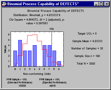
The binomial distribution fit is not statistically significant, so we can conclude that the binomial distribution yields an acceptable fit to the data, although visual inspection shows that the sizeable deviations in the margins of the distribution. The observed PPM is 133,333; however, based on the binomial distribution fit, we could expect a PPM of approximately 49,518.
You may repeat this analysis using the Poisson distribution, which yields a slightly better fit to these data, and a similar estimate of process capability.
See also Process Analysis - Capability Analysis Binomial and Poisson and Capability Analysis - Binomial and Poisson - Computational Details.