Example 4: Mixed-Model Factorial ANOVA Design

For details concerning mixed models (designs with random effects), see the Introductory Overview; see also the Variance Components and Mixed Model ANOVA/ANCOVA module topics.

This example is based on a small data set presented in Milliken and Johnson (1992, p. 238), who analyzed the data set using a two-way factorial ANOVA, treating the main effects and the two-way interaction as random effects. They also estimated variance components using several different estimation methods.

Specifying the Analysis

To perform these analyses in STATISTICA, open the Mill238.sta data file and start the General Linear Models module:

Ribbon bar. Select the Home tab. In the File group, click the Open arrow and select Open Examples to display the Open a STATISTICA Data File dialog box. The Mill238.sta data file is located in the Datasets folder. Then, select the Statistics tab. In the Advanced/Multivariate group, click Advanced Models and from the menu, select General Linear to display the General Linear Models (GLM) Startup Panel.

Classic menus. From the File menu, select Open Examples to display the Open a STATISTICA Data File dialog box. The Mill238.sta data file is located in the Datasets folder. Next, from the Statistics - Advanced Linear/Nonlinear Models submenu, select General Linear Models to display the General Linear Models (GLM) Startup Panel.

Select Factorial ANOVA as the Type of analysis and Quick specs dialog as the Specification method. Then click the OK button to display the GLM Factorial ANOVA Quick specs dialog box.

Click the Variables button to display the standard variable selection dialog box for factorial ANOVA designs. The dependent variable is DV and the categorical predictor variables are A and B. Select DV from the Dependent variable list, A and B as Categorical predictors (factors), and then click the OK button. A dialog box may be displayed to inform you that some of the variables contain text labels. Click the Continue with current selection button to close it and return to the GLM Factorial ANOVA Quick specs dialog box.

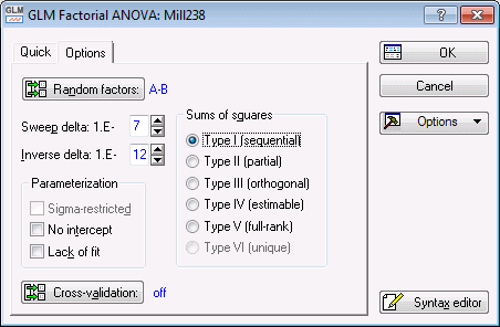
Select the Options tab. Click the Random factors button to display the Random Effects (Mixed Model) dialog box.

Select A and B as random factors, and click the OK button to return to the GLM Factorial ANOVA Quick specs dialog box.

Note: the Sigma-restricted check box under Parameterization has automatically become unavailable. This is because the overparameterized coding of categorical predictor variables is always used for mixed-model analyses (i.e., analyses that include random effects in the between design; see also Variance Components and Mixed Model ANOVA/ANCOVA).

One analysis that Milliken and Johnson (1992) performed used Type I decomposition of the sums of squares, so select the Type I option button under Sums of squares.

The remainder of the specifications for this analysis can use the default specifications, so click the OK button to perform the analysis. Note that the syntax program automatically generated from the specifications is:

Results.

Type I estimates of variance components

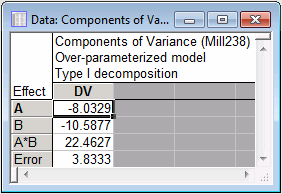
In the GLM Results dialog box, select the Summary tab. Click the Var. comps. button to create a spreadsheet containing the estimated components of variance for DV.

Within rounding, these estimates agree with those presented by Milliken and Johnson (1992, p. 239).

Type III estimates of variance components

Milliken and Johnson (1992) also estimated variance components using Type IV sums of squares. Type IV estimates for data with no missing cells also correspond to Type III estimates and to Type V estimates.

To obtain these estimates, click the Modify button in the GLM Results dialog box to return to the GLM Factorial ANOVA Quick specs dialog box. (Note that if you return first to the GLM Analysis Syntax Editor, click the < Back button to return to the GLM Factorial ANOVA Quick specs dialog box.)

On the Options tab, select the Type V option button under Sums of squares (Type III or Type IV could also be selected), and then click the OK button to perform the modified analysis. When the GLM Results dialog box is displayed, select the Summary tab and click the Var. comps. button to display the Type V variance component estimates.

Again, these estimates agree with those presented by Milliken and Johnson (1992, p. 239). Note that for both sets of estimates, the variance components for A and B are estimated to have negative values. This is one of the disconcerting features of variance component estimation - estimates are quite often negative. In practice, negative variance components are usually treated as indicating a 0 (zero) component, and thus are not necessarily problematic. Therefore, both sets of estimates clearly agree in suggesting that the A by B interaction effect represents the only nonzero component of variation in the dependent variable (other than Error).

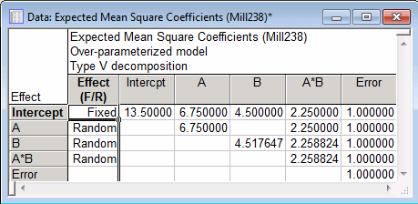
To test the significance of effects in designs involving random effects, error terms must be constructed that contain all the same sources of random variation except for the variation of the respective effects of interest. This is done using Satterthwaite's method of denominator synthesis (Satterthwaite, 1946), which finds the linear combinations of sources of random variation that serve as appropriate error terms for testing the significance of the respective effects. The covariation between sources of variation is represented by the elements in the Expected Mean Squares Coefficients matrix, which can be produced by clicking the Expected MSs button.

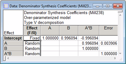
Click the Denom synth. button to display the Denominator Synthesis Coefficients spreadsheet containing the coefficients used to construct the linear combinations of sources of random variation based on Type V sums of squares.

The coefficients show, for example, that the Mean square for A should be tested against .996094 times the Mean square for the A by B interaction, plus .003906 times the Mean square for Error.

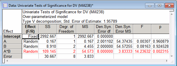
To perform the tests of significance, ratios of appropriate Mean squares are formed to compute F statistics and p-values. Click the All effects button to display the summary table for the mixed-model ANOVA.

As shown in the Univariate Tests of Significance for DV spreadsheet, the A by B interaction effect is found to be significant at p < .05, but neither the A main effect nor the B main effect approach significance, F's < 1.0. Note also that the A main effect has fractional denominator degrees of freedom, reflecting the synthesized error term used to test its effect. The B main effect has 2 denominator degrees of freedom, because it is tested solely against the A by B interaction effect with 2 degrees of freedom. The intercept cannot be tested because it has 0 degrees of freedom for its synthesized error term.

See also GLM - Index.