Weight of Evidence (WoE) example

This example illustrates how the Weight of Evidence (WoE) module can be used in an analysis project for risk assessment. Input a set of predictor variables into the analysis to find optimal coding for both continuous and categorical variables. Their resulting weight of evidence can be used as continuous inputs for Logistic Regression, improving that model’s performance.

  • Data file: CreditRisk.sta
  • Variable of interest: Credit Standing: Good or Bad
  • Goal of the analysis project: To classify credit applicants in terms of their Credit Standing

To distinguish between Good and Bad Credit Standing, you will use several independent (or predictor) variables, including the following:
  

Categorical Variables Continuous variables
  • Checking Acct
  • Credit Hist
  • Purpose
  • Savings Acct
  • Employment
  • Gender
  • Personal Status
  • Housing
  • Job
  • Telephone
  • Foreign
  • Monthly Acct
  • Residence Time
  • Age.

A combination of the independent predictor variables may help to explain Credit Standing. They can be used to build a predictive model to classify new customers.

Before building such a model, use the Weight of Evidence tool to

  • Recode the variables into discrete categories
  • Assign each category a value for WoE.

You can then use the WoE values as continuous predictors for the logistic regression model.

Open the CreditRisk.sta data set

1 Select the File tab. The File screen displays with a menu down the left side.
2 Click Open Examples in the left hand menu. The Open a Statistica Data File dialog box displays.
3 Open the Datasets folder. The datasets located in the  Datasets folder display.
4 Double-click CreditRisk.sta spreadsheet. The spreadsheet displays.

Start the Weight of Evidence module

  Select the Home tab. The Home tab ribbon opens, displaying the File, Output, Tools, SharePoint and Windows groups.
1 Select the Data Mining tab on the ribbon. The DataMining options display on the ribbon.
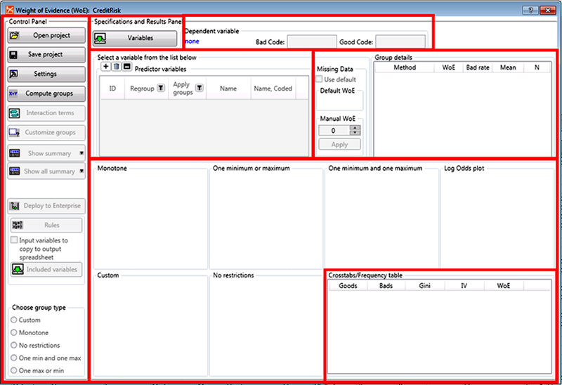
2 In the Tools group, click Weight of Evidence. The Weight of Evidence (WoE) dialog box displays.
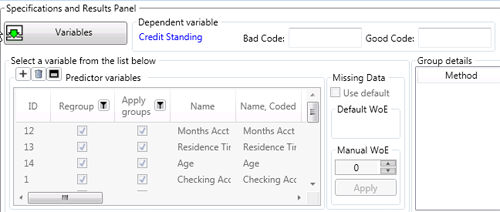
3 In the Specifications and Results Panel (top), click the Variables button.

The Select the variables for the analysis dialog box displays.

4 Select the Show appropriate variables only check box. The selection of variables displayed changes, as this option filters the variable lists according to their Measurement Type.

For more information see Select Variables.

5 Select the following variables:  
  • 15 - Credit Standing as the Dependent variable
  • 12, 13, and 14 as the Continuous Predictor variables
  • 1 through 11 as Categorical Predictor variables
6 Click the OK button.   The Variables dialog box will close and two areas of the WoE dialog box will populate:
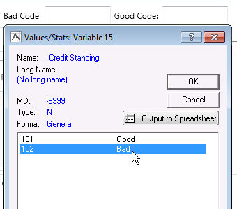
  • The Dependent variable group box will update with the selected variable Credit Standing
  • The Predictor variables dialog box will populate with the Continuous and Categorical Predictors.
7 Double-click in the Bad Code field. The Values/Stats dialog box displays.
8 Select Bad and click OK. The Bad Code and Good Code fields will update.

Compute groups

1 In the Control Panel (the left pane), click the Compute groups button to compute the best default coding solution for all variables. A Generating results status bar displays. The dialog box will update with the calculated weight of evidence information.
  • The Predictor variables box  activates.
  • Missing Data activates and populates.
  • Group details populates.
  • The Custom and No restrictions graphs display.
  • The Crosstabs/Frequency table populates.
2 Click the Show all summary button in the Control Panel. A drop-down list displays.
3 Select All coding in the menu to produce output for each variable. The results  produced are  consistent with the chosen preferences in the Options dialog box - Output Manager tab.

By default the results are placed  into a workbook as called Workbook1*.

  • In the workbook, a folder is created for each predictor variable.
  • The output gives an overview of the calculated recoding of each input variable for all appropriate methods

.

4 Select the folder for the variable Age, and review the results. The first output, the All Groups Summary for Age, shows the six methods used to compute age boundaries, the weight of evidence, and boundary values:
  • Monotone
  • One minimum or maximum
  • One minimum and one maximum
  • Custom
  • No restrictions
  • Log Odds plot

Only the graphs with solutions will display in the list.

5 Back in the Weight of Evidence (WoE) dialog box, click on Age in the Predictor variables group to display the charts for that variable. The same graphs for the Age predictor that display in the Workbook display in the dialog box. Note that the one not listed displays with No Solution.

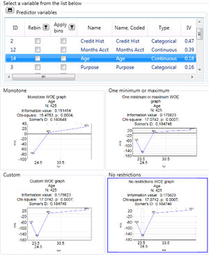
Weight of Evidence Graphs

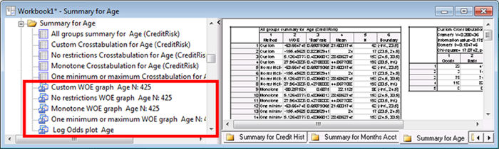
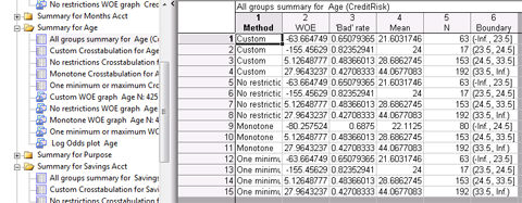
The following screen shot shows the WoE graph for the Custom method for the variable Age.
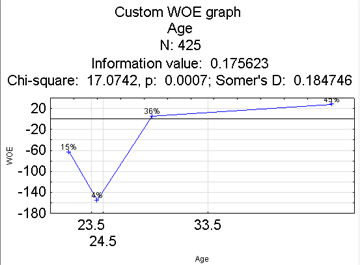
This plot shows:

  • Age across the x axis. The labels on the x axis denote the boundaries of the groups that were calculated with this method.
  • WoE on the y axis

Each point is labeled with the percent of cases found in this  grouping.

This plot shows four groups of average ages:

  • 21.6
  • 24
  • 28.7
  • 44

A small category, from Age 23.5 to 24.5, represents only 4% of cases and has a much lower WoE than any of the other groups. It's WoE is also much lower than any of the others.

Why is the Weight of Evidence so different for this group?

Two possible scenarios could cause these results:

  • Customers who are 24 years old might really have a very different Credit Standing than customers in the other  age categories.
  • By random chance,  a greater number of Bad Credit Standing customers might just happen to be present in this sample.

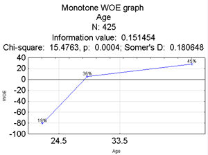
Look at the WoE from a different perspective to see which scenario is most likely true.

Use the Monotone method to find a different solution.  

1 Under Summary for Age in the workbook, select the Monotone WOE Graph to explore a different grouping.

This WoE graph contains only the following three groups instead of four:

  • From 18 to 24.5,
  • From 24.5 to 33.5
  • 33.5 and above

The Information value of 0.15, indicates that this variable has a medium strength relationship with the Y outcome, Credit Standing.

Conclusion: The WoE of the age group from 23.5 to 24.5, which is  found in several of the other methods,  is likely a data anomaly and not a real relationship of interest. This simpler grouping seems more logical

2 In the Control Panel of the WoE dialog box, in the Choose group type box at the bottom, select the Monotone option button,  to use this grouping.

Creating custom groups

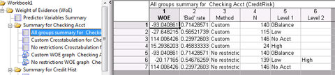
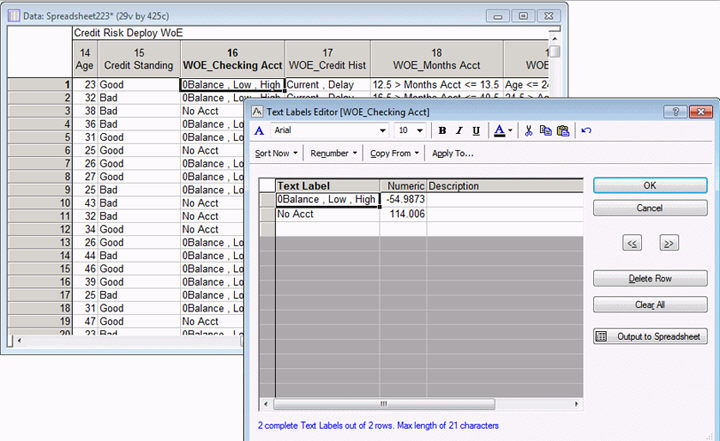
Next, explore the variable Checking Acct.
  

1 Click the icon the to left of the Predictor variables header to enlarge that pane.

The Predictor variables pane will expand to display more of the list. In this example, all variables will display..

2 Select Checking Acct, and click the icon by the header again to display the pane at its smaller size.

The graphs and output in the Weight of Evidence (WoE) dialog box will update for the selected variable. Since Checking Acct is a categorical variable, some methods are not valid and their panes display No Solution.

The Custom solution and the No restrictions solution are both shown. In the Group details pane (top right), you can see that the Custom solution does not combine any of the Checking Acct groups and they are all listed separately.

  • Custom (0Balance)
  • Custom (Low)
  • Custom (No Acct)
  • Custom (High)
  • No restrictions (0Balance
  • No restriction (Low), (High)
  • No restrictions (No account)

The No Restrictions method groups Low and High are the only ones grouped. The others remain in individual groups.

For ease of use, two groups, No Acct or Any Acct, encompassing 0Balance, Low, and High, would work better.
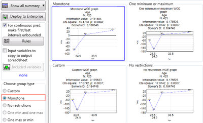
3 In the Control Panel, in the Choose group type box, select the Custom option. The Custom graph is highlighted.
4 Then, click the Customize groups button up in the main Control Panel. The Customize Groups for a Categorical Variable dialog box displays.
5 Select 0Balance, Low, and High.
6 Click the Group button. Notice how the Custom WoE graph changes.
7 Click OK. The Customize Groups dialog box closes. The graphs and Group details group update.
8 In the Control Panel, click the Show Summary button. A list will display.
9 Select All coding. The workbook updates. Under Summary for Checking Account, the Custom Crosstabulation for Checking Acct output shows information about the new grouping of this variable.

The overall Information Value is 0.596, which means that this variable is a strong predictor of Credit Status. Even with customizing the split, this variable can still contribute significantly to the final logistic regression model.

Deployment via Enterprise

Note: The remainder of this example can be followed only by those who have the Statistica Decisioning Platform software.

If you are happy with the remaining default groupings, the solution is ready for deployment.

1 In the WoE dialog box, in the Control Panel, click the Deploy to Enterprise button. The Select the required variables for creating rules dialog box will display. The buttons at the bottom will prompt you to either Deploy all variables or Deploy only selected variables. A Cancel button also displays.
2 Choose Deploy all variables. The Choose Deployment Type dialog box will display.
3 Ensure that the Deploy New Object option is selected, and click the OK button. The Select a Data Configuration dialog box will display. The None checkmark at the bottom will be selected by default, and the dialog box will be inactive.
4 Deselect the None checkbox. The dialog box will become active.
5 Navigate to the Credit Risk WoE folder and open the Credit Risk data configuration.  Click OK.
Note: If you do not see the data configuration, follow the directions at then end of this example to create one. The data configuration (in this case) queries the CreditRisk.sta example data set.

If SDMS is enabled, the Reason box will display

6 If the Reason box displays, fill it out and click OK to advance

The Enter a name dialog box will display.

7 Ensure the name Credit Risk 1 is entered into the Enter a name dialog box.
8 Click OK. A Statistica Enterprise permission dialog box will display.
9 Select the data configuration, and click OK. The Enter Object Name dialog box displays.
10 Enter Credit Risk Deploy WoE in the Enter name box and click OK. The Access Permissions dialog box will display.
11 Click OK. A prompt is displayed with options for the Enterprise object.
12 Click OK to accept the default setting so that the object uses the same placement and permissions as the data configuration. The WoE deployment object is added to Statistica Enterprise.
13 Click the OK button. The Success dialog box goes away.
14 Open Statistica Enterprise Manager to view this object.

Navigate to System View/Statistica Enterprise/Credit Risk Deploy WoE/.

The form will display.
15 Run the analysis by right clicking the Credit Risk Deploy WoE analysis object and selecting Run from the shortcut menu. As the analysis configuration runs, the data are queried and new WoE variables are added to the spreadsheet. The result is a spreadsheet with 14 new variables containing the new grouping strategies with Weight of Evidence values.
16 Back in Statistica , review the text labels.
    1. Select the Data tab.
    1. In the Variables group, click Specs.
The Variable1 dialog box displays.
17 Cancel the variable specification dialog box.  
18 Click Text Labels in the Variable group on the ribbon. The Text Labels Editor. displays. The numeric value is the weight of evidence value. The text that shows in the spreadsheet comes from the grouping.  
19 Click Cancel in the Text Labels Editor. The Text Labels Editor will close. The data are now ready to be used as input for logistic regression analysis.

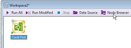
Deployment via the Workspace

Additionally, Weight of Evidence Rules can be deployed in the Statistica Workspace. The rules must first be saved as an *.srx file.

1 In the Weight of Evidence (WoE) dialog box, in the Control Panel, click the Rules button. The Select the required variables for creating rules dialog box will display.
2 Review the rules, which are listed as a series of if/then/else conditions.    
3 Click the Save button, and from the menu, select Save to File. The Save as dialog box displays.
4 Click the Cancel button in the  Save as dialog box and in the Rules Builder. The dialog boxes close.
5 In Statistica, click the File menu, then New and the Workspace icon. The Create New Document dialog box opens
6 Under Workspace Template, select Enterprise.  
7 In the file list, select Blank and click the OK button. The dialog box closes and the Select Data Source dialog box displays.
9 Click the Enterprise Data button. The Select Enterprise data configuration dialog box will display.
10 Select the appropriate data configuration and click OK to add it to the workspace.

The workspace will display with the node in it.

11 Click  Node Browser  in the Workspace.

The Node Browser dialog box will display.

12 Ensure All Validated Procedures is selected in the top drop-down list, and navigate to All in the left pane. You will see all validate procedures listed in the right pane.
13 Select the Rules node in the right pane.
14 Click the icon to insert the selected node into the workspace.

The node is inserted into the workspace.

15 Close the Node Browser dialog box.  
16 Double-click the Rules node in the workspace. The Rules dialog box displays.
17 Click the Edit button in the Rules group box..   The  Rules Builder displays
18 Click the Open button.
19 Select Open from file. The Open dialog box displays.
20 In the Open dialog box, browse to the *.srx file saved previously, select it, and click the Open button.  
21 Click OK in the Rules Builder to update the selection.  
22 In the Edit Parameters dialog box, select the True option button for Output a spreadsheet. Leave the rest of the option buttons at their default settings (as shown in the next image).  
23 Click the green arrow button adjacent to the Input variables to copy to result spreadsheet edit field.  
24 In the Select Variables dialog box, click the Select All button.  
25 Click the OK button.
26 Click the OK button in the Edit Parameters dialog box. The box closes.
27 In the workspace, click the Run icon The workspace runs, and the workspace is updated with a results workbook and spreadsheet containing the deployed WoE rules. The spreadsheet Credit Risk can be used as input for logistic regression analysis.

Using Deployment Results for Logistic Regression

1 Double-click the Credit Risk spreadsheet in the workspace. The Select dependent variables and predictors dialog box displays.
2 Click the Variables button. A variable selection dialog box displays.
3 Select Credit Standing as the Dependent, categorical variable.  
4 Select the newly created WoE variables as Predictor, continuous.
5 Click the OK button. A prompt  displays, stating that variables with text labels are selected as continuous variables.
6 Click the Continue with current selection button.  The WoE values  will be used for analysis.
7 In the Select dependent variables and predictors dialog box, select the Always use these selections, overriding any selections in the generating node may make check box.  
8 Click the OK button.  
9 Display the Node Browser again to add the Generalized Linear Models analysis node to the workspace, which is found in the Generalized Linear and Nonlinear Models folder (a subfolder of Statistics/Advanced Linear and Nonlinear Models).
10 Select Generalized Linear Models, and click Insert into workspace.  
11
    1. Double-click the GLZ node to display the Edit Parameters dialog box:
      • Change the Distribution to Binomial.
      • Change the Link Function to Logit.   
12 Click OK. The Edit Parameters dialog box closes.
13 Click Run. The workspace project runs and the logistic regression model builds, using the WoE results.
14 Double-click the Generalized Linear Models node to review the results.  

Create the CreditRisk.sta data set

Note: You will only need these instuctions if you are deploying to Enterprise and the Credit Risk WoE folder is not already present on your system.
  Create a system folder. Example 1: Setting Up the System View
  Create a database connection Example 3: Setting Up a Database Connection
  Create a data configuration under the folder you created in step 1. Example 4: Setting Up a Data Configuration