Example 2: Breakdown and One-Way ANOVA
Overview. You can compute various descriptive statistics (e.g., means, standard deviations, correlations, percentiles, etc.) broken down by one or more categorical variables (e.g., by Gender and Region) as well as perform a one-way Analysis of Variance via the Breakdown and one-way ANOVA procedure accessible from the Basic Statistics and Tables dialog box.
Open the example data file Adstudy.sta for this example, and start the Basic Statistics and Tables module.
Ribbon bar. Select the Home tab. In the File group, click the Open arrow and on the menu, select Open Examples. The Open a Statistica Data File dialog box is displayed. Adstudy.sta is located in the Datasets folder. Select the Statistics tab. In the Base group, click Basic Statistics to display the Basic Statistics and Tables dialog box.
Classic menus. From the File menu, select Open Examples to display the Open a Statistica Data File dialog box; Adstudy.sta is located in the Datasets folder. From the Statistics menu, select Basic Statistics/Tables to display the Basic Statistics and Tables dialog box.
Select Breakdown and one-way ANOVA and click the OK button.
In the Statistics by Groups (Breakdown) dialog box, select the Individual tables tab. Click the Variables button to display a variable selection dialog box.
Select Measure01 through Measure23 as the Dependent variables, and the two variables Gender (subject's gender, Male and Female) and Advert (type of advertisement shown to the subjects, Coke and Pepsi) as the Grouping variables, and click OK.
Click the Codes for grouping variables button to display the Select codes for indep. vars (factors) dialog box, and select all codes for both of the grouping variables. To select all codes for a variable, you can either enter the code numbers in the respective edit field, click the respective All button, or enter an asterisk * in the respective edit field. Clicking the OK button without specifying any values is equivalent to selecting all values of all variables.
Click the OK button in this dialog box and in the Statistics by Groups (Breakdown) dialog box to display the Statistics by Groups - Results dialog box, which provides various options and procedures for analyzing the data within groups in order to obtain a better understanding of the differences between categories of the grouping variables.
Summary Table of Means. You can select the desired statistics to be displayed in the Summary: Table of statistics or Detailed two-way tables; select the Descriptives tab and select all the check boxes in the Statistics group box. Click the Detailed two-way tables button to display the results spreadsheet.
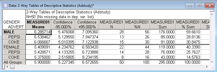
This spreadsheet shows the selected descriptive statistics for the variables as broken down by the specified groups (scroll the spreadsheet to view the results for the rest of the variables). For example, looking at the means within each group in this spreadsheet, you can see that there is a slight difference between the means for Males and Females for variable Measure01. Now, examine the means within the Male and Female groups for variable Measure01; you can see that there is very little difference between the groups Pepsi and Coke within either gender; thus, the gender groups appear to be homogenous in this respect.
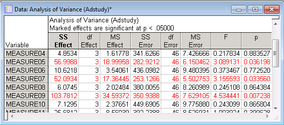
One-Way ANOVA and Post-Hoc Comparisons of Means. You can easily test the significance of these differences via the Analysis of Variance button on the ANOVA & tests tab. Click this button to produce the spreadsheet with the results of the univariate analysis of variance for each dependent variable.
The one-way analysis of variance procedure gave statistically significant results for Measure05, Measure07, and Measure09. These significant results indicate that the means across the groups are different in magnitude. Now, return to the Results dialog box and select the Post-hoc tab to perform post-hoc tests for the significant differences between individual groups (means).
You will first need to select the variable(s) for the comparisons. For this example, click the Variables button, select variable Measure07, and click OK. You can choose from among several post-hoc tests (an even larger selection of tests is available in the GLM module); for this example, click the LSD test or planned comparison button.
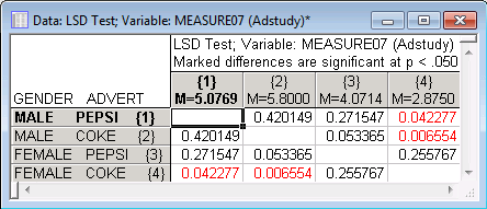
The LSD test is equivalent to the t-test for independent samples, based on the N in the groups involved in the comparison. The t-test for independent samples results from Example 1 showed that there was a significant difference between the responses for Males and Females for Measure07. Using the breakdown and one-way ANOVA procedure, you can see from the LSD test that a significant difference occurs only when the females are shown the Coke advertisement.
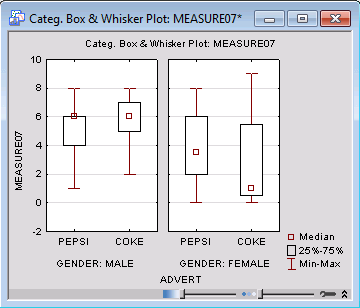
Graphical presentation of results. These differences can be viewed graphically via the many graphic options in the Statistics by Groups - Results dialog box. For example, to compare the distributions of the selected variables within the specified groups, select the Descriptives tab and click the Categorized box & whisker button. In the Box-Whisker Type dialog box, ensure that the Median/Quart./Range option button is selected, and click the OK button. Select the appropriate variable(s) to produce the graphs. Shown below is the box-whisker plot for variable Measure07.
As you can see in the above box and whisker plot for variable Measure07, there does appear to be a difference in the distribution of values for the Female-Coke group as compared to the Male-Coke group.
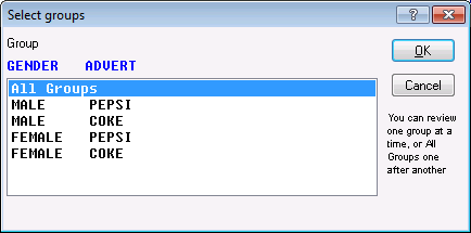
Within-Group Correlations. Now we will look at the correlations between variables within the specified groups. Return to the Statistics by Groups - Results dialog box, and select the Correlations tab. Note that numerous options are available on this tab to display various statistics and auxiliary information, in addition to the (within-group) correlation matrices. For this example, change the p-value for highlighting option to .001. Then, click the Within-group correlations & covariances button. The Select groups dialog box is displayed, in which you can select one group (or All Groups) for the correlation matrices.
In Example 1, a correlation matrix was produced in which the correlation between variables Measure05 and Measure09 (r = -.47) was highly significant (p<.001). The breakdown and one-way ANOVA procedure enables you to explore this significant correlation further by computing correlations within the specified grouping variables.
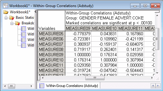
In the Select groups dialog box, select All Groups and then click the OK button to produce all four correlation matrix spreadsheets.
As you can see, the results reveal that the pattern of correlations is differentiated across the groups (e.g., the correlation is very high in the Female/Coke group and much lower in the other three groups). None of the correlations between Measure05 and Measure09 were significant at the .001 level; however, if you were to change the p-value for highlighting field to .05 on the Correlations tab of the Results dialog box, and click the Within-group correlations & covariances button again, you would find that the correlation between Measure05 and Measure09 is significant at that level (p=.02) for the group defined by Female gender and Coke advertisement.
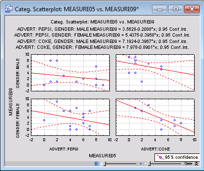
Categorized scatterplots. The within-group correlations can be graphically presented via the Categ. scatterplots button on the Correlations tab of the Statistics by Groups - Results dialog box. When you click this button, you will be prompted to select the variables for the analysis. Select Measure05 in the First variable list and Measure09 in the Second variable list and then click the OK button to produce the plot.
The above categorized scatterplot clearly shows the strong negative correlation between Measure05 and Measure09 for the group Female/Coke.
See also, the Basic Statistics and Tables Index and Overviews.


