Example 5: Standardized Solutions for the Effect of Peer Influence on Ambition
In a standardized solution, the latent variables all have unit variance. Setting the variances of exogenous latent variables to unity is trivial, because (a) these variances can be specified directly as part of a model, and (b) they are essentially arbitrary. Endogenous latent variable variances are a different matter. In some structural modeling programs, there is no convenient way to constrain the endogenous latent variables. For such programs to produce a standardized solution, a two stage procedure is employed. First, model parameters are estimated with the variances of the endogenous variables identified (at some unspecified value). After iteration is complete, the standardized coefficients are computed, using well known results from the algebra of multiple linear regression to transform the variances of endogenous latent variables to unity.
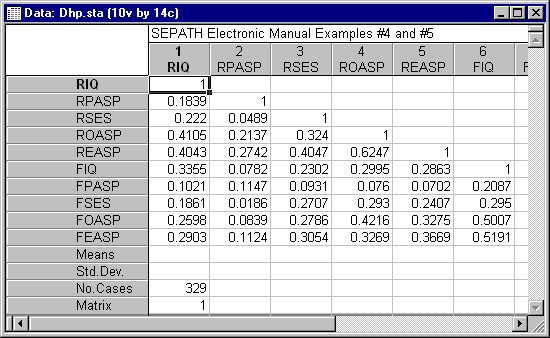
To produce such an old fashioned standardized solution, analyze the data in Dhp.sta.
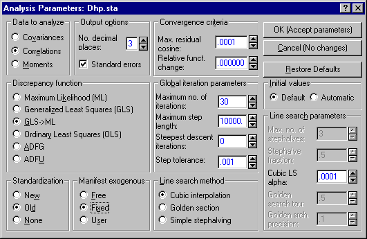
On the Analysis Parameters dialog, select the Fixed option button under Manifest exogenous, and select the Old option button under Standardization.
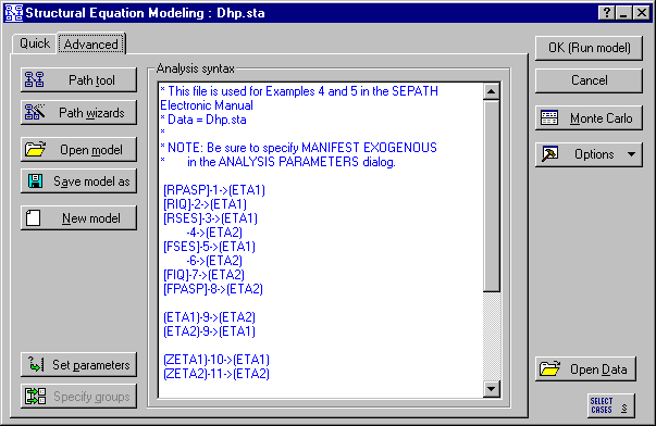
Use the model in Dhpa.cmd.
Execute the estimation, and compare the results with the unstandardized solution. One point is particularly noteworthy here. Some of the constraints that were specified for the unstandardized model are violated in the standardized model. For example, the path coefficients to ROASP and FOASP that were fixed at 1.0 in the unstandardized model now have values of .767 and .771, respectively. This is because the post hoc adjustment that produces the standardized coefficients simply employs the (unstandardized) numerical values and some regression algebra. The procedure is not "aware" of any equality constraints on parameters, and cannot be guaranteed to maintain them.
This would appear to create no real problem, since the values were assigned an arbitrary value of 1.0 simply to identify the variances at some value. On the other hand, two paths were constrained to be equal (those with the coefficient label 9 in the path diagram) for reasons other than identification purposes. These no longer have equal values in the standardized model estimates.
There is a third issue that is probably already obvious to the reader after comparing standardized and unstandardized solutions. Standard errors are not provided in the "old" standardized solution. This is because the post hoc adjustment of the unstandardized coefficients produces values whose information matrix is not the same as that for the unstandardized values.
We have established three major points so far:
- The "old" approach to standardization produces the same discrepancy function as obtained in the unstandardized solution.
- Equality constraints on the parameters imposed on the unstandardized solution may not be maintained when the parameters are transformed to the standardized form.
- Standard errors are not available with the Standardization - Old option.
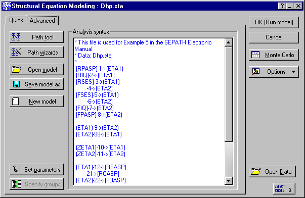
Now, we will explore the properties of the new standardization approach. This approach uses constrained estimation to force endogenous latent variables to have variances of one. Consequently, fixed parameter values of one that were used to identify the variances of endogenous latent variables should now be changed to free parameters before employing the Standardization - New option.
Open Dhpa.cmd and find the following section of the model.
(ETA1)-12->[REASP]
-->[ROASP]
(ETA2)-->[FOASP]
-13->[FEASP]
Change the fixed coefficients to free parameters, so the revised paths look like this:
(ETA1)-12->[REASP]
-21->[ROASP]
(ETA2)-22->[FOASP]
-13->[FEASP]
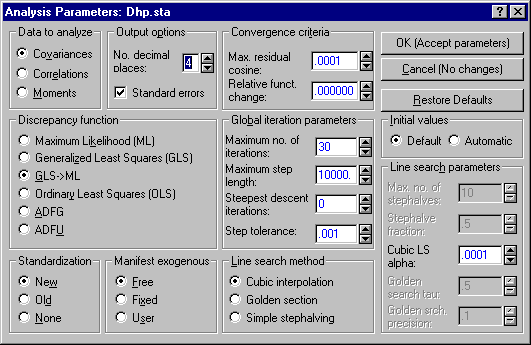
On the Analysis Parameters dialog, select the Free option button under Manifest exogenous, and select the New option button under Standardization. Also, under Output options, set No. decimal places to 4.
Execute the iteration, and observe the results. You will notice that the Chi-square statistic for the model is slightly lower than it was for the unstandardized solution (26.8964 to 26.8987). This is because the Standardization - New option produces standardized coefficients by constraining the estimation process. All equality constraints you imposed in your model are maintained during estimation. Notice that the two coefficients constrained to be equal (those with the parameter number 9) are estimated to be the same number. In the Standardization - Old procedure, these are not actually equal once the post hoc standardization procedure is employed. This demonstrates an important point that is often lost in discussions of standardization. Because constraints imposed on the unstandardized solution are usually not maintained in the standardized solution, the Chi-square statistic obtained in the old standardization approach may not, in fact, be correct. Another way of putting it is that the "old" standardization approach may remove your model constraints without your consent. Some of these constraints may have been artificial ones designed to achieve identification. However, if the constraints have some important substantive purpose, you should be aware that the "old" standardization approach may remove them.
The Lagrange multiplier statistics for the variance constraints are an important diagnostic tool for assessing whether model constraints were serving merely to achieve identification or were accomplishing some other purpose. In this case, we have removed two constraints on model coefficients. These constraints forced two parameters to be equal to a fixed value of one. We have now removed these constraints, and if forcing latent variable variances to be unity imposes no further constraints on the model fitting process, we should see two indications.
- The Chi-square statistic for the model in the Standardization - New option should be the same as in the Standardization - Old option.
- LaGrange multiplier statistics for all standardization constraints should all be zero.
We see that, in this case, both indications are not present. We have already noted that the Chi-square statistic is slightly different than in the Standardization - Old solution. The LaGrange multiplier statistics are slightly greater than zero, indicating that the standardization of latent endogenous variables actually imposes constraints on this model.
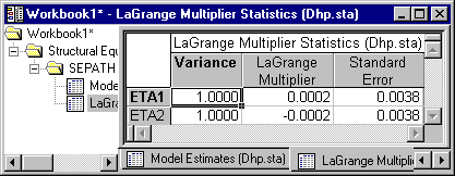
If the unit variances were simply an identification condition (as they frequently are) these statistics would all be zero. But in this case, imposing the standardization restriction on the endogenous latent variables constrains the solution for the path coefficients. The value of the coefficients that minimizes the discrepancy function, subject to the standardization constraints, is not one of the solutions that is a global minimum when the latent variable variances are unconstrained.
The problem is that the constraints on the variances of the latent variables interact with the constraint on the two coefficients labeled 9. If we allow the two paths labeled with coefficient 9 to vary freely, by renumbering one of them 99, we find a slightly lower Chi-square value, and zero Lagrange multiplier statistics (input for this example is in the file Dhpa3.cmd). For this solution, the coefficients will not agree with the old fashioned output produced by the commands in Dhpa.cmd.
The old fashioned output was obtained by standardizing, after the fact, coefficients that were generated under the constraint that the two paths between ETA1 and ETA2 are equal. Standardization after the fact invalidates that constraint, but the solution will not be the same as it would be if you relaxed the constraint, computed a solution, and then standardized. If, however, you return to the original input file (Dhpa.cmd), relax the equality constraint for the two paths labeled with coefficient number 9, and recompute, you will find that the standardized coefficients and Chi-square statistic agree precisely with those computed by the new method with the commands in Dhpa3.cmd. Note that the new procedure allows standard errors to be calculated, while the old procedure does not.
Let us briefly review the points covered in the preceding examples.
- The old fashioned approach to standardization has one advantage - computational simplicity. However, confidence intervals for standardized parameters cannot be calculated with this method. Moreover, equality constraints and fixed value constraints that are satisfied by coefficients in the unstandardized solution may not be satisfied in the standardized solution.
- When converting an old model to the new standardized method, you should free up parameters that were fixed solely for the purpose of identifying the variances of endogenous latent variables. There should be one such parameter for each endogenous latent variable.
- If Lagrange multiplier statistics are not zero, relax all equality constraints on parameters, and double-check to make sure you have freed up the parameters that were fixed for identification purposes.
- If your solution has a significant number of manifest exogenous variables, you can speed up iteration using the Manifest exogenous Fixed option, then restart the iteration with the Manifest exogenous Free option after convergence has occurred in order to guarantee correct standard errors and Chi-square values.
- In the previous examples, we analyzed a covariance matrix as though it was a correlation matrix in order to remain consistent with traditional analyses of the data. Consequently, standard errors are not generally correct. The program gave warning messages before computing its results.
By selecting the Correlations option button under Data to Analyze on the Analysis Parameters dialog, you can obtain a fully standardized path model with correct standard errors.
