Example 1: Automatic selection of the best number of clusters from the data
- Overview
- This example is based on a classic example data set reported by Fisher (1936), which is widely referenced in the literature on discriminant function analysis. The Statistica Discriminant Function Analysis module Examples also discuss an analysis using this data set. The data set contains the lengths and widths of sepals and petals of three types of irises (Setosa, Versicol, and Virginic). The purpose of a discriminant function analysis using this data set usually is to learn how you can discriminate among the three types of flowers based on the four measures of width and length of petals and sepals. In this example, it is illustrated how the methods for determining the best number of clusters from the data, available in the Generalized EM and k-Means Cluster Analysis module of Statistica, can be used to identify the different types of iris if you do not know a priori that those three types exist.
In other words, suppose you only have the measurements for 150 different flowers of type iris, and are wondering whether these flowers "naturally" fall into a certain number of clusters based on the measurements available to you. In more general terms, suppose you have a set of measurements taken on a large sample of observations, and you are wondering whether any clusters of observations exist in the sample, and if so, how many. Thus, this type of research question will come up in various domains, such as marketing research where one might be interested in clusters of lifestyles or market segmentations; in manufacturing and quality control applications, one might be interested in any clusters or patterns of failures or defects occurring in the final product (e.g., on silicon wafers), etc.
Specifying the analysis
- Data file
- The data file for this analysis is Irisdat.sta. A partial listing of the file is shown below. Open this data file via the File - Open menu; it is in the /Examples/Datasets directory of STATISTICA.
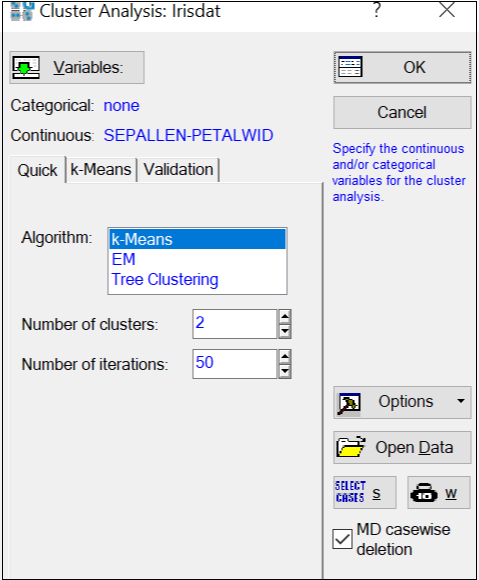
Open the Cluster Analysis (Generalized EM, k-Means & Tree) module by selecting that command from the Data Mining menu. In the Cluster Analysis dialog box, click the Variables button. In the variable selection dialog box, select as continuous variables in the analysis variables 1 through 4: Sepallen, Sepalwid, Petallen, and Petalwid. Note that we are not selecting variable Iristype. Click the OK button. Consistent with the stated purpose of this example (see the Overview paragraph above), we will instead pretend that we have no prior knowledge regarding the "true" number of clusters (types of iris) contained in the data set.
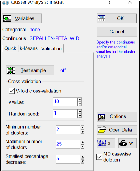
- Specifying v-fold cross-validation
- Click on the
Validation tab, and select the V-fold cross-validation check box. As explained in the
Introductory Overview (see also the description of the
Validation tab), this technique will divide the sample of 150 flowers into v "folds" or randomly selected samples of approximately equal size. STATISTICA will then perform repeated cluster analyses for each v-1 samples (i.e., leaving out one sample), and classify (assign to clusters) the observations in the sample that were not used to compute the respective cluster solution. That sample will be treated as a test sample, for which the average distance of observations from their respective (assigned) cluster centers will be recorded. This measure of "misclassification error" or "cost" will be averaged over all v replications of the analysis. STATISTICA will continue to perform these computations for increasing numbers of clusters until in successive cluster solutions (with k and k+1 clusters) the percentage decrease in the misclassification error is less than the Smallest percentage decrease, specified on the Validation tab; at that point, k will be taken as the best number of clusters for the data.
Now, click OK to perform the computations and display the Results dialog.
Reviewing Results
Note that, as discussed in the Introductory Overview, the results of your analysis may be different because the initial random assignment of observations (based on the random number seed) is different; you can enter the same random number seed (as shown in the above illustration) to achieve the same results.
In this particular case, the program extracted 4 clusters from the data.
- Graph of cost sequence
- Let us first look at the Graph of the cost sequence. As described in the
Introductory Overview as well as the
Results - Quick tab topic, this graph depicts the error function (average distance of observations in testing samples to the cluster centroids to which the observations were assigned) over the different cluster solutions.
It appears that the error function quickly drops from the 2- to the 3-cluster solution, and then it "flattens" out. Using the same logic as applied to the similar Scree plot computed in Factor Analysis (for determining the best number of factors), you could choose either the 3 or the 4-cluster solution for final review. For this example, let's accept the 4-cluster solution selected by the program.
- Graph of continuous variable means
- Click the Graph of continuous variable means button to display a line graph that shows the scaled cluster means for all continuous variables. These means are computed as follows:
where
 is the transformed (scaled) mean for continuous variable i and cluster j
 is the arithmetic ("unscaled") mean for continuous variable i and cluster j
 are the maximum and minimum observed values for continuous variable i
In other words, the plotted values depict the means scaled to the overall ranges of observed values for the respective continuous variables.
It appears that the pattern of means for Cluster 1 is quite distinct from that for the other clusters. You can also click the Cluster distances button to verify that the distance of Cluster 1 from all the others is larger than the distances between clusters 2, 3, and 4.
- Other results
- You can now review in detail the patterns of means for the variables in this analysis and the distribution of cases assigned to the different clusters. These typical results of interest in k-Means clustering are described in greater detail in the Cluster Analysis Overviews and in Example 2.
- Comparing the final cluster solution with actual iris types
- For this example, we deliberately ignored variable Iristype, i.e., the previous knowledge we had regarding the true number of clusters in the sample. It is interesting to review how "well" we did with the cluster analysis, in identifying the real iris types. In other research applications, it might be of interest to find appropriate labels for the final clusters by running additional analyses to relate the cluster assignments to other variables of interest. In this case, we will simply compute a crosstabulation table of the cluster assignments by the actual Iristype recorded in the Irisdat.sta data file.
On the Results dialog - Quick tab, click the Save classifications & distances button, and then select Iristype as an additional variable to save along with the cluster analysis results (assignments, distances to cluster centers). Part of the resulting data file is shown below.
This data file will automatically be created as an input file for subsequent analyses (see also option Data - Input Spreadsheet). Select Basic Statistics/Tables from the Statistics menu, select Tables and banners to display the Crosstabulation Tables dialog, and then compute a cross tabulation table of variable Iristype by Final classification.
Shown above is the summary crosstabulation table, along with the (row) percentages of observations of each known Iristype classified into the respective clusters. As expected, Cluster 1 (the one that showed the greatest distance from all others) is most distinct. 100% of all flowers of type Setosa were correctly classified as belonging to a distinct group or cluster. Cluster 3 and Cluster 4 apparently identify the flowers of type Versicol and Virginic that are easily "classifiable," while Cluster 2 contains both flowers of type Versicol and Virginic. It appears that these two types of flowers are not as easily distinguished, a result that is consistent with those that were computed in the Discriminant Function Analysis - Example.
Summary
The purpose of this example is to illustrate the usefulness of the Generalized EM and k-Means Cluster Analysis module for automatically determining a "best" number of clusters from the data, using v-fold cross-validation techniques. This extension of traditional clustering methods makes it a very powerful technique for unsupervised learning and pattern recognition, which are typical tasks encountered in Data Mining.