Response Optimization Example - Classification

Applying the Simplex Algorithm: In this step-by-step example, we demonstrate the use of Statistica Response Surface Optimization using the data set IrisSNN.sta. The example involves a classification problem in which the predicted or dependent variable is FLOWER with categorical levels Setosa, Versicol, and Virginic.

Procedure

  1. Open the file IrisSNN.sta via the File > Open Examples menu; it is in the Datasets folder.
  2. Select Response Optimization for Data Mining Models from the Data Mining - Process Optimization submenu.

    Click the Load models button to display the Open PMML files dialog box and load the following .xml files from the Examples/Datasets folder: Iris1, Iris2, Iris3 (select these files and click the Open button). These .xml files contain trained Multilayer Perceptron Neural Networks saved in PMML language.

  3. Upon loading the predictive models, the Response Optimization module is automatically set the options to default values. These values are calculated from various statistics of the appropriate variables in the data set, such as mean, variance, minimum, and maximum. For example, the descriptive statistics of the independent variables are used to initialize the starting values, step sizes, and range on the Simplex tab of the Simplex algorithm. However, you may need to modify some of these default values as they might not always be the best choice for your particular analysis. For instance, you may need to change the desired categorical response value on the Quick tab to a setting of your choice. The default is usually the first of the categorical levels' list in the PMML file.
  4. Particularly useful information that you can display in spreadsheet format is the descriptive statistics of the variables. You can do so by clicking the Variables button in the Response Optimization Startup Panel. This information helps you to select sensible option settings for your analysis. For example, the minimum and maximum of the variables can help you to decide on the settings of the Simplex, Grid, and Random algorithms . By setting the minima and the maxima of the Simplex algorithm, for instance, equal to the minimum and the maximum of the appropriate variables in the data set, you can in fact confine the Simplex search to regions of the independent space that was spanned by the original data set. This confinement is important since optimization may lead to unreliable results should it be conducted outside regions falling way off the boundaries of the original data set.
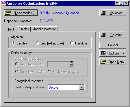
  5. Let's now find a set of independent values for which the categorical response level Setosa has the highest confidence. To do this, set the Seek categorical level option that is located in the Optimization type group box on the Quick tab to Setosa.
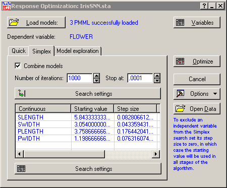
  6. select the Combine models check box on the Simplex tab. Models combined to cooperate on making predictions are called ensembles, which are known to have a better generalization ability (i.e., to predict unseen data more accurately).
  7. Next, click the Optimize button in the Startup Panel. This will initiate the Simplex algorithm. While the algorithm is in progress, a progress bar will be displayed showing the progress of the algorithm. When the search is complete, several outputs in the form of spreadsheets and graphs will be displayed.
    The first graph is the line plots of all models' confidence levels for Setosa (y-axis) against iteration number (x-axis).

    Since you combined the models, a second graph will be displayed containing the same information as the first graph, but for the ensemble.


  8. By reviewing this graph (which contains one plot per model), you can tell if the algorithm has succeeded in finding the desired categorical level, and how many iterations it took to converge. Note that the same information displayed in this graph can also be viewed in the form of a spreadsheet (Iterations, simplex search spreadsheet).

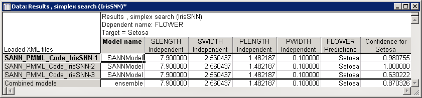
    Another output, the most important one, is the results spreadsheet. Here you can view the final solution found by the algorithm, i.e., the set of independent values for which the ensemble yielded maximum confidence for classifying Setosa.

  9. Note that you can repeat the same optimization for any categorical level of your choice. In our next search, we may, for example, want to find a Simplex solution for which the confidence levels for Versicol is the highest. Do this by selecting this category from the drop-down menu of the Seek categorical level option in the Categorical response group box on the Quick tab.

The Grid Method

The Simplex technique is a guided optimization algorithm that can find the desired solution in a finite number of steps.

However, just as any other algorithm, sometimes it may not find the desired solution. In cases such as this, you can use the Grid or Random algorithms, which are implementations of simple techniques based on brute computing power. For instructions on using the Random algorithm, see the step-by-step example for regression.

Here is an example for using the Grid method.

As before, we want to find the attributes of the Iris flower for which model predictions yield maximum confidence for Setosa.

Procedure

  1. select the Grid (exhaustive) option button on the Quick tab and set the desired value of Seek categorical level option to Setosa.
  2. Before starting the optimization, you may want to review the default settings of the Grid algorithm, such as starting and end values, as well as step sizes. To change these values, click the Search settings button on the Grid tab. This displays a standard STATISTICA user input spreadsheet.
  3. After modifying the settings displayed in the spreadsheet, click OK to make the new settings permanent.
  4. Now, click the Optimize button. Upon completion of the algorithm, two spreadsheets are displayed. The first contains the settings of the Grid algorithm; the second spreadsheet contains the best result found by the Grid search.