Example 1: Transformation of Variables
General Conventions and Options
In these examples, the general conventions used in the Time Series module to maintain the active work area (which functions as a queue of successive transformations of the input series; refer to Active Work Area) will be reviewed. Thus, transformations or the results of other analyses can be undone, saved, etc.
Transformations and the Active Work Area
Specifying the Analysis
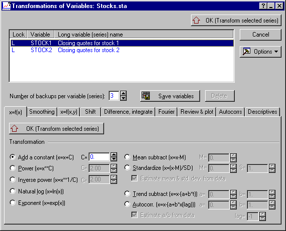
To start the analysis, select Time Series/Forecasting from the Statistics - Advanced Linear/Nonlinear Models menu to display the Time Series Analysis Startup Panel. Then, click the Variables button to display the standard variable selection dialog. Here, select variables Stock1 and Stock2 and then click the OK button. The opening dialog of the File module will now look like this.
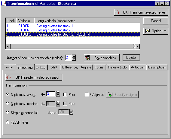
All variables (series) and their transformations that are currently available for analysis are stored in the active work area and are listed in the scrollable edit fields at the top of the dialog. When you select new variables, the active work area will first be cleared, and then the selected variables will be read into the active work area (after all "holes" with missing data have been "patched;" see below and Active Work Area).
Highlighted variable
All subsequent analyses will be performed on the highlighted variable. For example, when you perform a transformation, then the currently highlighted variable will be transformed, and a new (transformed) variable will be appended to the active work area. To highlight a variable, simply click on it in any of the scrollable edit fields. For this example, highlight the variable Stock1.
Naming conventions
When a new (e.g., transformed) variable is appended to the active work area, it is assigned (1) the same short variable name as the original variable (that was transformed), and (2) a new long variable name that consists of the old long variable name (as much of it as will fit) and a brief description of the respective transformation that was performed. In this manner, as you perform successive transformations or analyses (e.g., successively difference a series), an automatic log of transformations will be maintained in the long variable names.
Editing variable names
Double-click in the column labeled Variable or Long variable (series) name to edit the short or long variable name for the series in the active work area. Note that the short and long names will only be changed in the active work area, not in the file (use the respective data spreadsheet operations to permanently change those names; see Variable Specs).
Number of backups per variable (series)
All dialogs that contain the scrollable edit fields for highlighting a variable (series) for an analysis also contain a field for specifying the desired Number of backups per variable (series). As described above, after a transformation (or other analysis) is performed on a series, the resulting transformed series (or residuals, forecasts, etc. in ARIMA) will be appended to the active work area, and the values of the series prior to the transformation will be maintained as a backup. The number of such backups that will be maintained in the active work area is controlled by this parameter. Thus, for example, if this parameter is set to 3, and you have just performed the fourth transformation of an original variable, then the series with the data after the first transformation will be dropped from the active work area and replaced by the new (fourth) transformed series. Thus, series created by successive transformations will be appended to the active work area until there are as many backups as specified in this parameter; at that point the respective "oldest" transformed series will be replaced by the new one. Up to 99 backups can be kept of a single original variable. For this example, accept the default value of 3 backups.
Locking variables (series)
The first column of the scrollable edit fields carries the header Lock. When you double-click in that column for a transformed variable, that variable will be locked in the active work area (or unlocked, if it was previously locked). An L will appear in that column to indicate that the variable is now locked. Locked variables will not be replaced as successive transformations exceed the current maximum number of backups (as described in the paragraph above). Note that original (untransformed) variables are always locked, and they cannot be unlocked.
Deleting variables (series) from the current work area
To delete a transformed variable from the active work area, use the Delete highlighted variable button. Original (untransformed) variables cannot be deleted.
Saving variables (series) in the current work area
Use the Save variables button to save the variables (series) in the active work area. You can save all variables or only selected variables.
Missing Data
Overall mean
In this method, all missing data will simply be replaced by the overall mean of the series. Very often, when the series is not stationary (see Introductory Overview), or when there are large systematic fluctuations in the values of the series, this method may not be appropriate. On the other hand, the overall mean is often the best a priori (unbiased) guess for the missing data.
Interpolation from adjacent points
In this method, the missing data are computed by interpolation from the adjacent non-missing points. Graphically, this method amounts to replacing missing data by connecting with a straight line the point just prior to the missing data with the point just following the missing data. Thus, this method in a sense assumes that there is some serial correlation in the data, that is, that each observation is to some extent related to and therefore most similar to the previous observation.
Mean of N adjacent points
In this method the missing data are computed from the mean of the N adjacent points on both sides of the "hole" of missing data. For example, when N is left at its default value of 1, then missing data will be replaced by the average of the value just prior to the missing data and the value immediately following the missing data. In general, this method implies that the data in the region or window specified by the N parameter are more similar to each other than points that are further away.
Median of N adjacent points
This method is essentially the same as that described above, except that missing data are replaced by the median of the N non-missing adjacent points.
Predicted values from linear trend regression
In this method, STATISTICA will fit a least-squares regression line to the time series. The missing data will then be replaced by the values predicted by this regression line. This method implies that the most salient (or strongest) feature of the series is its linear trend across time.
Reviewing the Time Series
Now proceed with the analysis and review the closing quotes for the two series. Click the OK (transformations, autocorrelations, crosscorrelations, plots) button to display the Transformations of Variables dialog.
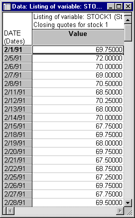
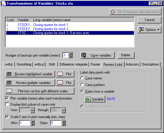
Several options for reviewing time series in the active work area are shown on Review & plot tab. The Label data points with box contains options that will determine how the horizontal (time) axis is scaled and labeled. Note that those options will affect all plots in the Time Series module (there are numerous options for plotting time series available with all procedures in the Time Series module). The example data file Stocks.sta contains dates in variable Date and in the case names and either of these can be used to label the horizontal axes in plots (select the appropriate option button).
You can plot this series by clicking the Plot button next to the Review highlighted variable button on the Review & plot tab.
To plot both stocks simultaneously, click the Plot button next to the Review multiple variables button, and then select the variables (series) to be displayed or plotted in the Select variables for the Spreadsheet/plot dialog. In this example, select both variables and then click the OK button.
Plotting Two Series with Different Scales
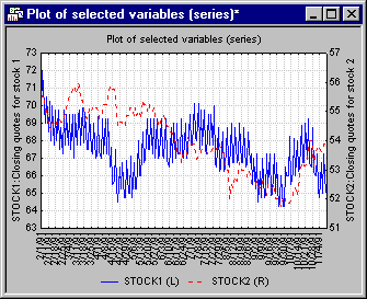
As you can see, the closing quotes for Stock2 are generally lower than those for Stock1. You can independently scale the vertical axes for those two series to obtain the best vertical resolution possible for each series. Click the Plot two var lists with different scales button and in the resulting Select variables for the Spreadsheet/plot dialog select to plot Stock1 against the left y-axis, and Stock2 against the right y-axis.This plot allows you to compare the pattern or movement of the two series across time more clearly.
Transforming Time Series
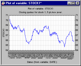
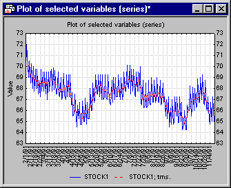
Now perform a few transformations. On the Transformations of Variables dialog, highlight the first series (Stock1). The various tabs on this dialog show all common transformations for time series data. Some of those transformations require that you select a second variable, for example, for Residualizing a time series via the x=f(x,y) tab. For this example, we will specify a simple (unweighted) 5-point moving average transformation for series Stock1 using the Smoothing tab. Select the N-pts. mov. averg. option button, and specify 5 as the window width in the N= box.Then, click the OK (Transform selected series) button, and the moving average transformation will be performed. When all cases have been transformed, then, by default (i.e., if the Plot variable (series) after each transformation check box is selected on the Review & plot tab), the transformed series will be plotted.
As you can see below, compared to the plot of the raw (untransformed) series (see above), the transformed series is much less "jagged," and the general trend over the trading days reflected by the data is much clearer.
Now return to the Transformations of Variables dialog.
The Updated Active Work Area
As described above, the transformed (smoothed) series has been appended to the active work area.
Following the naming conventions described earlier, the transformed variable has the same short name (Stock1) and will have the same long name, except that a brief description of the transformation (5 pt. mov. aver.) was added to the existing title. Note that if the original title had been much longer, so that the description of the transformation couldn't fit, then the original long variable name would have been deleted.
Further Processing of the Transformed Series
The transformed series in the work area has the same "status" as those series that were originally selected and read into the active work area from the file. For example, they can be plotted, saved, or used as input into further analyses. Now, compare the smoothed series with the original input series. On the Review & plot tab, click the Plot button next to the Review multiple variables button. By default, the original series and the smoothed series will be highlighted in the subsequent Select variables for the Spreadsheet/plot dialog.
Simply accept this default selection and click the OK button. Shown below is the joint plot of the raw input series and the smoothed (transformed) series.
Multiple Successive Transformations
Now, continue to transform the transformed variable and observe how successive series are appended to the active work area. Highlight the transformed series (the one at the bottom of the list) by clicking on it. For now, turn off the automatic graphing option, that is, clear the Plot variable (series) after each transformation check box. Then, click on the Smoothing tab and select the Simple exponential smoothing option button with the default parameter alpha = .20. Now, click the OK (Transform selected series) button and then select the 4253H Filter option button (this is a powerful smoothing/filtering technique that applies several moving average and moving median transformations in succession; refer to the Smoothing tab topic for details) and again click the OK (Transform selected series) button.
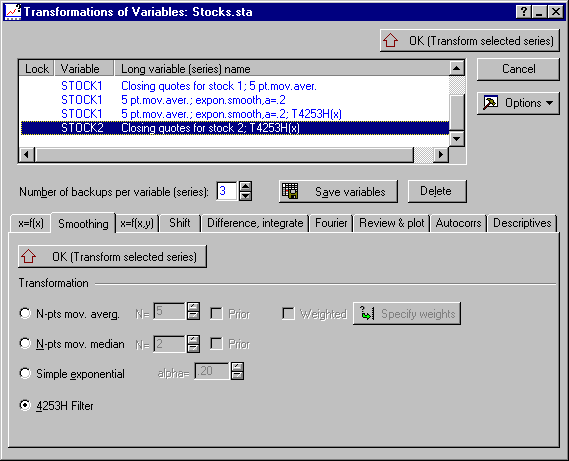
There are now 3 transformed series that were appended to the active work area. Assuming that you have not changed the Number of backups per variable (series) parameter from the default value of 3, the active work area is now "full." The next transformation of any of the variables derived from Stock1 will replace the "oldest" transformation for that variable. Thus, if you now transform variable Stock2, another (the first) backup of that variable will be added. Try this by applying the 4253H Filter to Stock2. (Select the Stock2 variable, make sure the 4253H Filter option button is selected and then click the OK (Transform selected series) button.) After the transformation is complete, the active work area will look like this.
As you can see, all transformations of variable Stock1 are still in place. However, now highlight the original variable Stock1 again (scroll the edit window until Stock1 is visible), and apply to it, for example, a 5-pt. mov. median transformation. (Select the N-pts mov. median option button on the and enter 5 in the corresponding N= box. Then click the OK (Transform selected series) button.) Now the "oldest" or first transformation that you performed on variable Stock1 (the 5-point moving average transformation) will be replaced by the 5-point moving median transformation of series Stock1.
Perhaps an appropriate "mental model" of the way in which series are managed in the active work area is that of a carousel: Successive transformations of a series are placed in successive positions of the carousel. The number of places on the carousel is determined by the Number of backups per variable (series) parameter . Once all places have been taken, then the next transformation will replace the first transformation, as the carousel starts the next go-around.
Locking
Suppose you would like to keep a transformation in the active work area; that is, you would like to prevent it from being replaced by another transformation.
To accomplish this, the respective transformation should be Locked: Double-click on the respective series in the Lock column, and an L will appear in the respective row of that column. The respective series is now locked; that is, it will not be overwritten by successive transformations of the same variable, or, put another way, it will stay in the same place on the carousel.
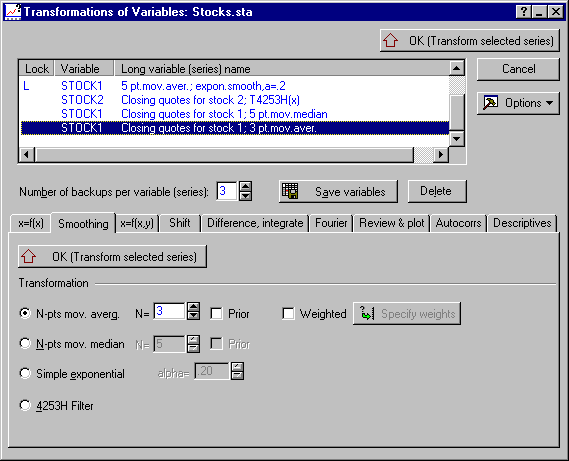
For example, the next "oldest" transformation of Stock1 that will be replaced is the Exponential smoothing transformation. Now, lock that series, then highlight the original Stock1 series again and apply to it a 3-pts. moving average transformation. (Select the N-pts mov. averg. option button, enter a 3 in the corresponding N= box, and click the OK (Transform selected series) button.) As you can see, the locked transformation was not overwritten.
Saving the Series in the Active Work Area
Now save the transformations in the active work area. Suppose you would like to keep only the 4253H transformations of Stock2 for further analysis. First, delete the series that you don't want to save from the active work area by highlighting them and then clicking the Delete button.
Then, save the variables in the active work area by clicking the Save variables button. You will be prompted for a file name under which STATISTICA will save all data currently in the active work area.
Autocorrelation Analysis
Thus far, the interpretation of the transformations has not been discussed. In general, the analysis of time series data requires a good deal of experience not only with the available techniques, but also with the nature of the data. For example, stock prices often follow what is called a random walk model. Simply stated, each observation is equal to the previous observation plus some random component. In a sense, the process behaves like "a drunken man whose position at time t is his position at time t-1 plus a step in a random direction at time t" (Wei, 1990, page 71). If so, you may expect that the simple autocorrelation is highest for a lag of 1, next highest for lag 2, etc., that is, that the autocorrelation function will show a slow decay. Put another way, the "drunken man" will be closest to where he was immediately before, a bit farther away from where he was before that, and so on. Technically, this process can be expressed as an auto-regressive process, with the autoregressive parameter (Ф in ARIMA terminology) approaching 1.0.
Plotting the Autocorrelation Function
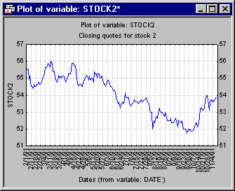
Now examine whether the closing quotes stored in Stock2 follow this simple model. First, plot Stock2 (highlight Stock2 and click the Plot button next to the Review highlighted variable button on the Review & plot tab).
It appears that Stock2 shows a downward trend. Such trends will bias the autocorrelation function; that is, if the stock is generally going down, then obviously, each quote will be more similar to the adjacent quotes as compared to those that are farther away.
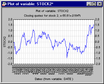
Therefore, you can detrend the series by clicking on the x=f(x) tab, selecting the Trend subtract option button, and then clicking the OK (Transform selected series) button. Now, if you plot the transformed variable again (by clicking the Plot button next to the Review highlighted variable button on the Review & plot tab), you can see that the trend was removed.
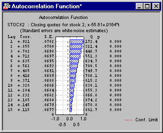
Now click the Autocorrelations button on the Autocorrs tab to display a spreadsheet and plot of the autocorrelation function.
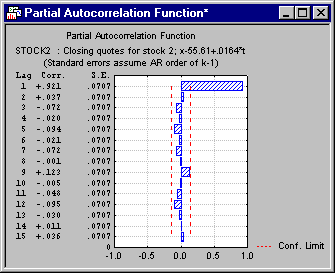
The correlation for lag 1 is large, and decays slowly thereafter; the plot of the partial autocorrelation function also supports the random walk model. (Click the Partial autocorrelations button to produce this plot.)
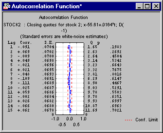
Above and beyond the very strong autocorrelation at lag 1, none of the partial autocorrelations are significant. Put into words, each observations is mostly similar to the previous observation, plus some random shock -- which represents the random walk model. You can "remove" the strong single autocorrelation by differencing the series. To do this, click on the Difference, integrate tab, select the simple Differencing (x = x-x(lag)) option button, and click the OK (Transform selected series) button. Then click the Autocorrelations button on the Autocorrs tab to produce the plot for the differenced series.
As you can see, none of the autocorrelations is significant. Thus, your initial guess from prior experience with the "behavior" of stock prices has been confirmed; Stock2 indeed follows the random walk model, and, unfortunately, given a particular quote at a particular time, there is no way to predict whether the stock will go up or down.
See also, Time Series Analysis Index.


