Example 4: Multinomial Linear Model with Generalized Logit Link
This example is based on the example data file Gator.sta (see Agresti, 1996, p. 214). The data are taken from a study by the Florida Game and Fresh Water Fish Commission of factors influencing the primary food choices of alligators. Fifty-nine alligators were sampled, their length was measured, and their primary food was determined. Data file Gator.sta contains the following variables:
Length: Length of the alligator (in meters)
Food: Primary food source (categorical dependent (response) variable with 3 categories: Inverteb, Fish, Other)
We will fit a multinomial linear model with a generalized logit link; variable Length is treated as the continuous predictor variable.
Open the Gator.sta data file in the following ways:
Ribbon bar. Select the Home tab. In the File group, click the Open arrow and from the menu, select Open Examples. The Open a STATISTICA Data File dialog box is displayed. Ideol.sta is located in the Datasets folder.
Classic menus. From the File menu, select Open Examples to display the Open a STATISTICA Data File dialog box; Ideol.sta is located in the Datasets folder.
- Specification of Model
- Start
Generalized Linear/Nonlinear Models:
Ribbon bar. Select the Statistics tab. In the Advanced/Multivariate group, click Advanced Models and from the drop-down list, select Generalized Linear/Nonlinear to display the Generalized Linear/Nonlinear Models Startup Panel.
Classic menus. From the Statistics - Advanced Linear/Nonlinear Models submenu, select Generalized Linear/Nonlinear Models to display the Generalized Linear/Nonlinear Models Startup Panel.
Select the Advanced tab, and select Simple regression as the Type of analysis, Quick specs dialog as the Specification method, Multinomial as the Distribution, and Logit as the Link functions. Then click the OK button to display the GLZ Simple Regression Quick Specs dialog box.
Click the Variables button to display the standard variable selection dialog. Select Food as the Dependent (response) variable, Length as the Continuous predictor variable, and then click the OK button. We can use all other default specifications, click the OK button to display the GLZ -- Results dialog box.
If you want to run this example using GLZ Syntax, you can run the following syntax program from the GLZ Analysis Syntax Editor dialog box (see Methods for Specifying Designs).
- Parameter Estimates
- On the
Summary tab, click the
Estimates button to review the parameter estimates.
Only the parameter estimates for category Inverteb are significant. Because in multinomial models, the last category is always the reference category (that is, the parameters pertain to the differences between the respective current category and the last category that was specified for the categorical response variable), this implies that the difference between the Invertebrates food type and the Other food type can be explained by Length, but the difference between the Fish food type and the Other food type cannot.
Next click the Goodness of fit button.
The model fits the data well, and there is no evidence of overdispersion since the ratios of the statistics over the degrees of freedom are all close to 1.0 (see also McCullagh and Nelder, 1989).
- Model Checking with Observational Statistics
- STATISTICA GLZ computes predicted values and residual statistics for each of the k-1 linear combination of predictors in the multinomial model with k categories.
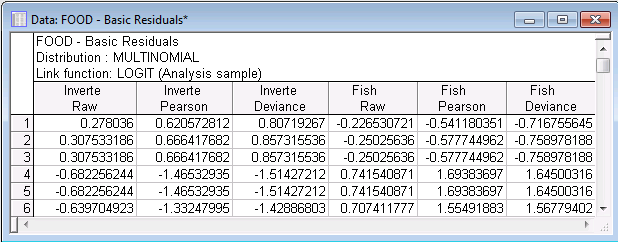
Select the Resid. 1 tab, and then click the Basic Residuals button to display raw residuals, Pearson residuals, and Deviance residuals for each observation and for each of the k-1 (non-reference) categories.
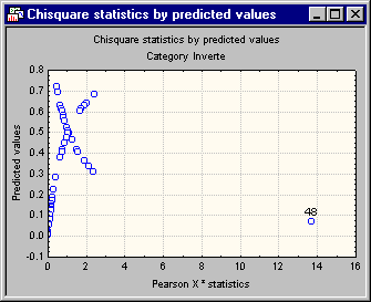
You can plot the Pearson Chi-square values (contributions to Chi-square) for each case against the predicted values for each (non-reference) category. To produce this plot, select the Resid. 2 tab, and then click the Pred. & Diff. X2 (Chi-square) button. You can see the plot for category Invertebrates.
In this example, the 48th data point (you can use the Brushing tools to label the outlier shown on the right side of the graph) has a large Chi-square value, and thus is the largest contributor to the lack of fit for this model. Removal of this point may yield different results. To accomplish this, all you need to do is go back to the data file, delete the data for the 48th case, and rerun the analysis.


