Example 6: Kruskal-Wallis ANOVA & Median Test
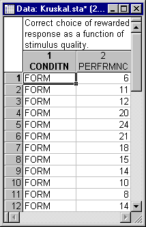
These tests are alternatives to one-way between-groups analysis of variance (ANOVA) (see the ANOVA module). Refer to the Nonparametric Statistics Notes - Kruskal-Wallis ANOVA by Ranks and Median Test topic for a discussion of the logic and assumptions of these tests. This example is based on a (fictitious) data set reported in Hays (1981, page 592), Kruskal.sta (a partial listing is shown below). Open this data file via the File - Open Examples menu; it is in the Datasets folder.
These data were obtained from small children who were randomly assigned to one of three experimental groups (treatments). Each child was shown a series of pairs of stimuli. Their task was to choose one of those stimuli, and, if it was the "correct" one, they received a reward. In one group, the relevant dimension that the children had to detect in order to make correct choices was form (group 1 - Form), in a second group the relevant dimension was color (group 2 - Color), and in the third group, the relevant dimension was size (group 3 - Size). The dependent variable was the number of trials that these children required to detect the relevant dimension that was being rewarded.
- Specifying the analysis
- Select Nonparametrics from the Statistics menu to display the Nonparametric Statistics Startup Panel.
Next, select Comparing multiple indep. samples (groups) from the Quick tab, and then click the OK button to display the Kruskal-Wallis ANOVA and Median Test dialog.
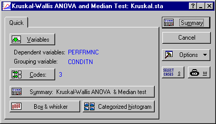
Click the Variables button to display the standard variable selection dialog. From the Dependent variable list, select variable Perfrmnc; as the Indep. (grouping) variable, select variable Conditn, and then click the OK button.
In the Kruskal-Wallis ANOVA and Median Test dialog, click the Codes button to display the Select codes for grouping variable dialog. Select all codes for the independent variable (by clicking the All button), and then click the OK button. The Kruskal-Wallis ANOVA and Median Test dialog will now appear as follows:
- Reviewing the results
- Now, click the Summary button to begin the analysis.
- Results of Kruskal-Wallis ANOVA
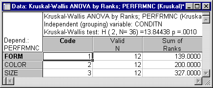
- The Kruskal-Wallis ANOVA by Ranks spreadsheet is displayed first, followed by the Median Test, Overall Medial spreadsheet.
The Kruskal-Wallis test is highly significant (p = .001). Thus, you can conclude that the performances of the different experimental groups were significantly different from each other. Remember that the Kruskal-Wallis test is basically an analysis of variance performed on ranks. The Sum of Ranks is displayed in the spreadsheet. The highest rank sum (worst performance) appears in the Size condition, that is, in the condition where children were rewarded for identifying size as the critical discriminating dimension; the lowest rank sum (best performance) appears in the Form condition.
- Results of Median test
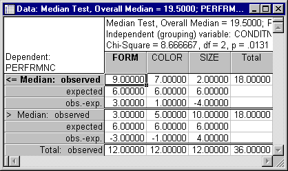
- The Median Test is also significant, however, less so (p = .013).
Remember that the Median test is more "crude" and less sensitive than the Kruskal-Wallis ANOVA (see the Nonparametric Statistics Notes - Kruskal-Wallis ANOVA by Ranks and Median Test topic). The spreadsheet shows the number of cases (children) in each experimental condition that fall below (or are equal to) the common median and the number of cases that fall above the common median. Again, the greatest number of subjects with above-median number of trials (below-median performance) are in experimental condition Size; the greatest number of subjects with below-median number of trials (above-median performance) are in experimental condition Form. Thus, this test confirms that the Form dimension was most easily recognized by the subjects, and the Size dimension was least easily recognized.
- Graphical representation of results
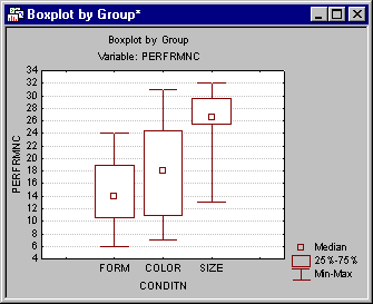
- Now, click the Box & whisker button in the
Kruskal-Wallis ANOVA and Median Test dialog. A standard variable selection dialog is displayed in which you need to specify the variable to be plotted. Select the Perfrmnc variable, and then click the OK button. Next, you will be prompted to select the statistics for the box plot in the
Box-Whisker Type dialog. For this example, select the Median/Quart./Range option button and then click the OK button to produce the plot.
Again, it appears that performance in the Form condition was better than in any other condition; the median number of trials in that condition is lower than in any other condition.
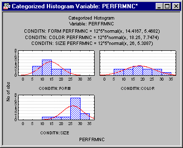
Another way to look at the distribution of the dependent variable within each condition is via the Categorized histogram button. Click this button in the Kruskal-Wallis ANOVA and Median Test dialog to produce this graph. Select the Perfrmnc in the variable selection dialog, and then click the OK button.
This graph again confirms that the performance in the Form category is "better" (i.e., the distribution is slightly skewed to the left) than in the other two conditions; performance clearly appears to be worst in the Size condition. Thus you can conclude that children most easily identified the Form dimension when it was rewarded.
See also, Nonparametric Statistics - Index.

