Special Topics Example 2 - Optimization of the Response Variable in a Three-Factor Mixture Experiment
- Overview
- This example describes how to profile predicted responses and response desirability in a mixture-experiment using the
Response/Desirability Profiler.
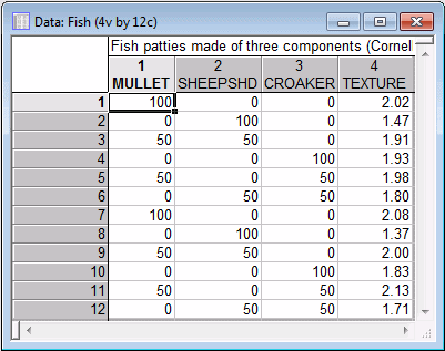
Example 8.1 described the design and analysis of Cornell's (1990a) simple but typical mixture experiment concerning the average texture of fish patties. Sandwich patties were made of blends of three types of fish: Mullet, Sheepshead, and Croaker. The dependent variable of interest was Texture, as measured by the force (in grams * 10-3) required to puncture the patty surface.
This example describes how to use the Response/Desirability Profiler to find the fish blend that produces patties with the most desirable texture.
- Design and coding of variables
- The analysis of these data begins in the same way as for any mixture design. The data discussed by Cornell (1990a) are contained in the example data file Fish.sta. Open this data file and start Experimental Design (DOE).
Ribbon bar. Select the Home tab. In the File group, click the Open arrow and from the menu, select Open Examples to display the Open a Statistica Data File dialog box. Double-click the Datasets folder, and open the Fish.sta data set. Then, select the Statistics tab, and in the Industrial Statistics group, click DOE to display the Design & Analysis of Experiments Startup Panel.
Classic menus. On the File menu, select Open Examples to display the Open a Statistica Data File dialog box. The Fish.sta data file is located in the Datasets folder. Then, on the Statistics - Industrial Statistics & Six Sigma submenu, select Experimental Design (DOE) to display the Design & Analysis of Experiments Startup Panel.
In the Startup Panel, double-click Mixture designs and triangular surfaces to display the Design & Analysis of Mixture Experiments dialog box.
Select the Analyze design tab, and then click the Variables button to display the variable selection dialog box.
Select Texture as the Dependent variable and Mullet, Sheepshd, and Croaker as the Independent vars (factors). Click OK in the variable selection dialog box, and click OK in the Design & Analysis of Mixture Experiments dialog box to display the Analysis of a Mixture Experiment dialog box.
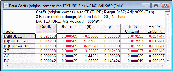
Cornell (1990a) fitted sandwich patty texture scores using a quadratic model, so select the Quadratic option button on the Model tab.
The fitted coefficients can be computed by clicking the Estimates, original components button on either the Quick tab or the Anova/Effects tab. The results from the Estimates original components spreadsheet is shown below (see also Example 8.1: Designing and Analyzing a Mixture Experiment).
The regression coefficients in the spreadsheet are used in computing predicted values for the dependent variable at different combinations of levels of the independent variables. Now, to profile the predicted responses and the desirability of responses, click the Response desirability profiling button on the Prediction & profiling tab to display the Profiler.
Response/Desirability Profiling
- Specifying the desirability function
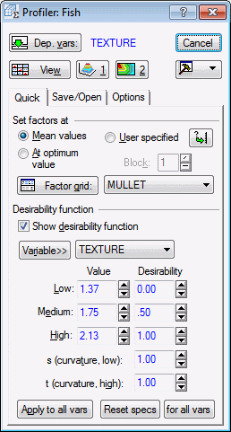
- Because we want to profile both the predicted responses on the dependent variable as well as the response desirability, the first step is to specify the desirability function for the dependent variable.
Ensure that the Show desirability function check box is selected to enable the edit fields for the Desirability function settings.
Cornell (1990a) specified that firmer fish patties are more desirable, so the default "higher is better" Desirability function settings can be left at their preset values of 1.37 (the lowest observed Texture score), 1.75 (the midpoint score), and 2.13 (the highest observed Texture score) in the low value, medium value, and high value edit fields, respectively. The corresponding default desirability values of 0.0, 0.5, and 1.0 are preset in the low desirability, medium desirability, and high desirability edit fields, respectively. Because Cornell's (1990a) suggested function between Texture and desirability does not imply any curvature in the "fall off" of desirability between "inflection" points, the values in the s parameter and t parameter edit fields can be left at their default values of 1.0, specifying linear changes in desirability between inflection points.
- Profiling the predicted responses and response desirability
- Click the View button to produce a compound response profile graph, using the factor means as the default current values for each predictor variable, and four steps from the observed minimum to the observed maximum to define the five default grid points for each factor.
A prediction profile for the dependent variable is shown, consisting of a series of graphs, one for each independent variable, of the predicted values for the dependent variable at each grid point of the independent variable, holding the levels of all other independent variables constant at their current values. By default, confidence intervals for the predicted values are also shown. A graph of the desirability function for the dependent variable is displayed, and a series of graphs, one for each independent variable, shows the profile of response desirability at each grid point of the independent variable, holding the levels of all other independent variables constant at their current values.
The overall desirability value of .78655 indicates that although the mean blend of equal amounts of each type of fish yields a sandwich patty with quite desirable Texture, an even more desirable product is possible.
A search for the levels of the ingredients that produce the most desirable product can be conducted. This can be specified by selecting the option button for the At optimum values in the Set factors at group box in the Profiler.
To conduct the search using a general function optimization method (the simplex method), select the Options tab, and select the Use general function optimization option button in the Search options (for optimum desirability) group box. Also, to display finer grids of predicted values and overall response desirability scores, click the Factor grid button on the Quick tab to display the Specifications for factor grid dialog box, and enter 20 for the No. of steps. Click the accompanying Apply to all button to specify a grid of 21 points for each independent variable. Click OK to return to the Profiler, and click the View button to produce a compound response profile graph, using the optimal values of the independent variables as their current values, and 20 steps from the observed minimum to the observed maximum to define the 21 grid points for each factor.
The results displayed in the compound response profile graph show that desirability is improved by setting the factors at levels other than their means. The overall desirability value is .92862 with the settings of Mullet, Sheepshead, and Croaker at 74.176%, 4.068%, and 21.754% respectively.
As an alternative method for conducting the search, select the Options tab, and select the Optimum desirability at exact grid points option button in the Search options (for optimum desirability) group box. Click the View button to produce a compound response profile graph, using the optimal values from the grid search as the current values for the independent variables.
The results displayed in the compound response profile graph show that the overall desirability value is .9285 with the settings of Mullet, Sheepshead, and Croaker at 75.0%, 4.1667%, and 20.833% respectively.
Further confirmation of the adequacy of the solution comes from returning to the Analysis of a Mixture Experiment dialog box (click Cancel in the Profiler) and click the Critical values (min, max, saddle) button on the Prediction & profiling tab. The critical values displayed in the resulting spreadsheet represent a maximum on the quadratic response surface. The values are 74.17619, 4.06859, and 21.75521 for Mullet, Sheepshead, and Croaker, respectively, all of which are quite close to the optimal values found by both search methods in the Response/Desirability Profiler.
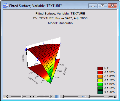
Surface plots and contour plots for predicted responses are available as options on the Prediction & profiling tab or the Quick tab. These same plots for response desirability are available as options in the Profiler. For this data set, the plots show that the surface is relatively flat near the maximum, meaning that small departures from the optimal settings for the independent variables would not appreciably decrease the desirability of the product.
- Summary
- This example has shown how to optimize a response variable in a mixture experiment. As an aside, but worth mentioning, some statistical packages do not take the mixture total constraint into account in response optimization procedures for mixture experiments. This can lead to at worst, misleading and at best, amusing results. It would seem to be a logical necessity that an all fish patty should contain 100% fish, no more and no less, and Statistica's Response/Desirability Profiler ensures that this logical necessity is met.