K-Nearest Neighbor Example 1 - Classification
In this example, we will study a classification problem, i.e., a problem with a categorical output (dependent) variable. Our task is to build a K-Nearest Neighbor classifier model that correctly predicts the class label (category) of the independent variables.
For the example, we'll use the classic Iris data set. This data set contains information about three different types of Iris flowers: Versicol, Virginic, and Setosa. The data set contains measurements of four variables [sepal length and width (SLENGTH and SWIDTH) and petal length and width (PLENGTH and PWIDTH)]. The Iris data set has a number of interesting features:
Procedure
- One of the classes (Setosa) is linearly separable from the other two. However, the other two classes are not linearly separable.
- There is some overlap between the Versicol and Virginic classes, so it is impossible to achieve a perfect classification rate.
Result
- Data file
- Open the IrisSNN.sta data file; it is in the /Example/Datasets directory of STATISTICA.
- Starting the analysis
- Select Machine Learning (Bayesian, Support Vectors, Nearest Neighbor) from the Data Mining menu to display the
Machine Learning Startup Panel.
Select K-Nearest Neighbors on the Quick tab, and click the OK button to display the K-Nearest Neighbors dialog. You can also double-click on K-Nearest Neighbors to display this dialog.
Click the Variables button to display a standard variable selection dialog. Select FLOWER as the Categorical dependent variable and variables 2-5 from the Continuous predictors (independent) variable list, and click the OK button.
At this stage, you can change the specifications of the analysis, e.g., the sampling technique (see the documentation for the Sampling tab) for dividing the data into examples and test samples, and the number of nearest neighbors K, as well as the distance measure (metric) and the averaging scheme (see the documentation for the Options tab). For analyses with more than one independent variable with significantly different typical values, you may also want to standardize the distances (for continuous independent variables only). For further details see below. The significance of the averaging scheme is also discussed below.
One important setting to consider is the sampling technique for dividing the data into examples and testing samples (on the Sampling tab). Although the choice of a sampling variable is not the default setting (as a sampling variable may not be available in your data set) you may want to use this option since it divides the data deterministically, unlike random sampling, which allows an easier comparison of results obtained with different experimental settings, i.e., choice of K, distance measure, etc.
For this example, on the Sampling tab, select the Use sample variable option button, and click the Sample button to display the Sampling variable dialog. On this dialog, click the Sample Identifier Variable button, select NNSET as the sampling variable, and click the OK button. Then, double-click in the Code for analysis sample field, select Train as the code for the analysis sample, and click the OK button. In the Status group box, click the On option button, and click the OK button.
When performing KNN analyses, it is recommended that you standardize the independent variables so that their typical case values fall into the same range. This will prevent independent variables with typically large values from biasing predictions. To apply this scaling, on the K-Nearest Neighbors dialog - Options tab, select the Standardize distances check box (this option is also available on the Results dialog).
Finally, select the Cross-validation tab. Select the Apply v-fold cross-validation check box; in the Search range for nearest neighbors group box, enter 30 in the Maximum field (to increase the maximum number of nearest neighbors K to 30).
Click the OK button. While KNN is searching for an estimate of K using the cross-validation algorithm, a progress bar is displayed followed by the K-Nearest Neighbor Results dialog.
- Reviewing results
- On the
K-Nearest Neighbors Results dialog, you can perform KNN predictions and review the results in the form of spreadsheets, reports, and graphs.
In the Summary box at the top of the Results dialog, you can see some of the specifications of your KNN analysis, including the list of variables selected for the analysis and the size of Example, Test, and Overall samples (when applicable). Displayed also are the number of nearest neighbors, distance measure, and whether input standardization and weighting based on distance are in use. You can also review the cross-validation error. Note that these are the specifications made on the K-Nearest Neighbors dialog.
On the Quick tab of the Results dialog, click the Cross-validation error button. This will create a graph of the cross-validation error for each value of K tried by the cross-validation algorithm.
The first thing you should look for in this graph is the existence of a saddle point, i.e., a value of K with maximum classification accuracy compared to its neighboring points. The existence of a maximum indicates that the search range for K was sufficiently wide to include the optimal (from a cross-validation sense) value. If it is not present, return to the KNN dialog by clicking the Cancel button on the Results dialog, and increase the search range.
As discussed before, STATISTICA KNN makes predictions on the basis of a subset known as examples (or instances). Click the Model button to create a spreadsheet containing the case values for this particular sample.
Further information on the classification analysis can be obtained by clicking the Descriptive statistics button, which will display two spreadsheets containing the classification summary and confusion matrix.
To further view the results, you can click the Predictions button to display the spreadsheet of predictions (and include any other variables that might be of interest to you, e.g., independents, dependents, and accuracy, by selecting the respective check boxes in the Include group box).
You can also display these variables in the form of histogram plots.
Further graphical review of the results can be made on the Plots tab, where you can create two- and three-dimensional plots of the variables and confidence levels.
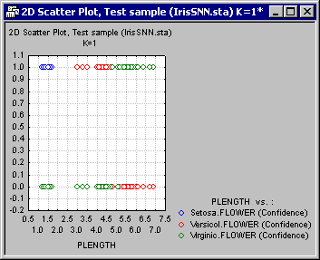
For example, shown above is a scatterplot of the independent variable PLENGTH against the confidence level of the categorical levels Setosa, Versicol, and Virginic. From the displayed (relative) values, it is clear that Setosa is well separated, while some degree of overlapping exists between Versicol and Virginic. This overlap accounts for the misclassified cases, which you can view from the predictions spreadsheet (see below). To produce the graph shown, in the K-Nearest Neighbors Results dialog, select the Test option button in the Sample group box, select PLENGTH from the X-axis list and Setosa (conf.), Versicol (conf.), and Virginic (conf.) from the Y-axis list. Then click the Graphs of X and Y button.
Note: you can determine the sample (subset) for which you want to display the results. Do this by making a selection from the Sample group box on the K-Nearest Neighbors Results dialog. For example, select the Overall option button to include both the examples and test samples in spreadsheets and graphs. However, note that you cannot make predictions (and other related variables, e.g., accuracy or confidence) for the examples sample since it is used by KNN for predicting the testing sample.Since there is no model fitting in a KNN analysis, the results you can produce from the Results dialog are by no means restricted to the specifications made on the K-nearest neighbors dialog. To demonstrate this, select the Options tab of the Results dialog, and clear the Use cross-validation settings check box. This will enable the rest of the controls on this tab, which are otherwise unavailable. (Note: This action will not discard the cross-validation results. You can always re-set your analysis to this setting by selecting the check box again). Change the number of nearest neighbors to 40.
On the Plots tab, select the independent variable PLENGTH as the X-axis and the confidence levels for the class levels (as before). Click the Graph of X and Y button. Note that due to the larger value of K (as compared to the cross-validation estimate 3) predictions have already started to deteriorate. You can easily see this by noticing the larger region of overlap between the class levels.
At this point, you may want to display a new descriptive statistics (Quick tab) spreadsheet for comparison with the previous one.
Indeed if you set K=80 (size of the examples sample) the performance of the KNN will reach its lowest. This is shown in the figure below.
Next, we'll study the effect of distance weighting on KNN predictions. Select the Options tab once again, and select the Distance weighted check box. Leave K at 80 and produce the graph of PLENGTH against the confidence levels once more. Despite the fact that all cases from the examples sample are included, there is significantly less overlap between the class levels. This implies a more correct classification is possible despite the inclusion of all cases belonging to the examples sample.
Finally, let's perform a "what if?" analysis. Select the Custom predictions tab.
Here, you can define new cases (that are not drawn from the data set) and execute the KNN model. This enables us to perform an ad hoc, "What if?" analysis. Click the Predictions button to display the prediction of the model.