Example 1: Factor Analysis
- Overview
- This example is based on a fictitious data set describing a study of life satisfaction. Suppose that a questionnaire is administered to a random sample of 100 adults. The questionnaire contains 10 items that are designed to measure satisfaction at work, satisfaction with hobbies, satisfaction at home, and general satisfaction in other areas of life. Responses to all questions are recorded via computer and scaled so that the mean for all items is approximately 100. The results for all respondents are entered into the Factor.sta data file.
Open this data file:
Ribbon bar. Select the Home tab. In the File group, click the Open arrow and on the menu, select Open Examples to display the Open a STATISTICA Data File dialog box. Open the Factor.sta data file, which is located in the Datasets folder.
Classic menus. On the File menu, select Open Examples to display the Open a STATISTICA Data File dialog box. Open the Factor.sta data file, which is located in the Datasets folder.
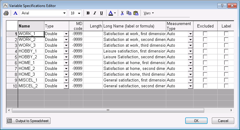
Following is a listing of the variables in the data file. To display the Variable Specifications Editor:
Ribbon bar. Select the Data tab. In the Variables group, click All Specs.
Classic menus. On the Data menu, select All Variables Specs.
- Purpose of the analysis
- The goal is to learn more about the relationships between satisfaction in the different domains. Specifically, it is desired to learn about the number of factors "behind" these different domains of satisfaction, and their meaning.
- Specifying the analysis
-
Ribbon bar. Select the Statistics tab. In the Advanced/Multivariate group, click Mult/Exploratory and on the menu, select Factor to display the Factor Analysis Startup Panel.
Classic menus. On the Statistics - Multivariate Exploratory Analysis submenu, select Factor Analysis to display the Factor Analysis Startup Panel.
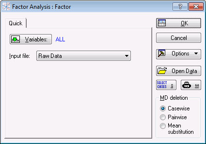
Click the Variables button, select all 10 variables, and click the OK button. The Startup Panel will look as shown below:
- Other options
- In order to perform a standard factor analysis, this is all that you need to specify in this dialog box. Note that you could also choose either Casewise or Pairwise deletion, or Mean substitution of missing data (via the MD deletion group box) or a Correlation Matrix data file (via the Input file option).
- Define method of factor extraction
- Click the OK button to display the Define Method of Factor Extraction dialog box. In this dialog box, you can review descriptive statistics, perform a multiple regression analysis, select the extraction method for the factor analysis, select the maximum number of factors and the minimum eigenvalue, and select other options related to specific extraction methods. For now, select the Descriptives tab.
- Review descriptive statistics
- Click the Review correlations, means, standard deviations button to display the
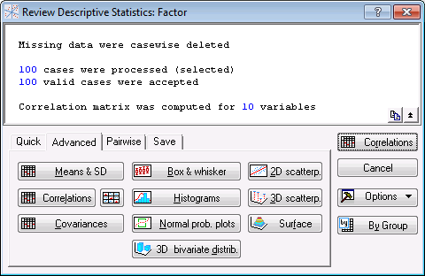
Review Descriptive Statistics dialog box. Select the Advanced tab.
Here, you can review the descriptive statistics graphically or through spreadsheets.
- Computing correlation matrix
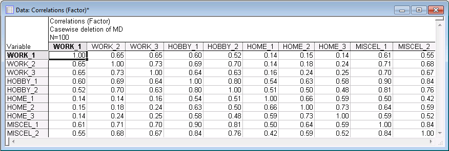
- Click the Correlations button to produce the Correlations spreadsheet.
All correlations in this spreadsheet are positive; some correlations are of substantial magnitude. For example, variables Hobby_1 and Miscel_1 are correlated at the level of .90. Some correlations (for example the ones between work satisfaction and home satisfaction) seem comparatively small. So, it looks like there is some clear structure in this matrix.
- Extraction method
- In the Review Descriptive Statistics dialog box, click the Cancel button to return to the
Define Method of Factor Extraction dialog box. You can choose from several extraction methods on the
Advanced tab (see
the Define Method of Factor Extraction - Advanced tab topic for a description of each method, and the
Introductory Overviews for a description of Principal Components and Principal Factors).
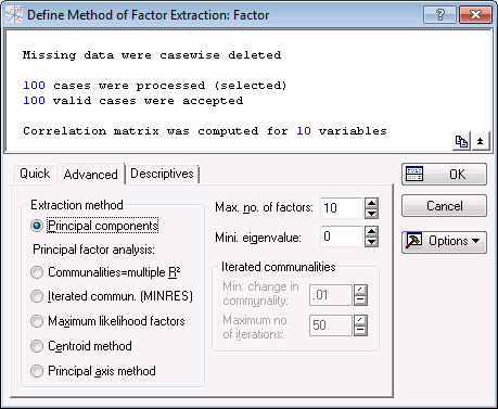
For this example, accept the default extraction method of Principal components and change the Max. no. of factors to 10 (the maximum number of factors in this example) and the Mini. eigenvalue to 0 (the minimum value for this option).
Click the OK button to continue the analysis.
- Reviewing results
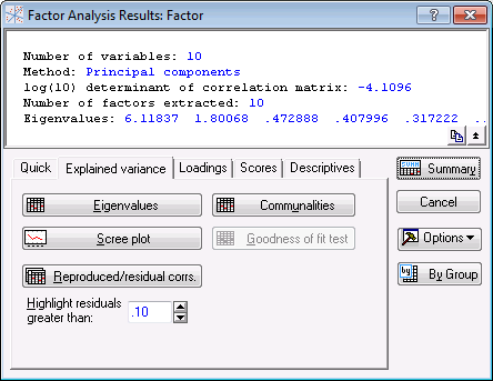
- You can interactively review the results of the factor analysis in the Factor Analysis Results dialog box. First, select the Explained Variance tab.
- Reviewing the eigenvalues
- The meaning of eigenvalues and how they help you decide how many factors to retain (interpret) is explained in the
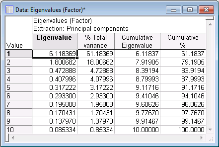
Introductory Overviews. Click the Eigenvalues button to produce the spreadsheet of eigenvalues, percent of total variance, cumulative eigenvalues, and cumulative percent.
As you can see, the eigenvalue for the first factor is equal to 6.118369; the proportion of variance accounted for by the first factor is approximately 61.2%. Note that these values happen to be easily comparable here because there are 10 variables in the analysis, and thus the sum of all eigenvalues is equal to 10. The second factor accounts for about 18% of the variance. The remaining eigenvalues each account for less than 5% of the total variance.
- Deciding on the number of factors
- The Introductory Overviews briefly describe how these eigenvalues can be used to decide how many factors to retain, that is, to interpret. According to the Kaiser criterion (Kaiser, 1960), you would retain factors with an eigenvalue greater than 1. Based on the eigenvalues in the Eigenvalues spreadsheet shown above, that criterion would suggest you choose 2 factors.
- Scree test
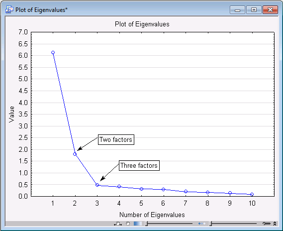
- Now, to produce a line graph of the eigenvalues in order to perform Cattell's scree test (Cattell, 1966), click the Scree plot button. The Plot of Eigenvalues graph shown below has been "enhanced" to clarify the test. Based on Monte Carlo studies, Cattell suggests that the point where the continuous drop in eigenvalues levels off suggests the cutoff, where only random "noise" is being extracted by additional factors. In our example, that point could be at factor 2 or factor 3 (as indicated by the arrows). Therefore, you should try both solutions and see which one will yield the most interpretable factor pattern.
Now, examine the factor loadings.
- Factor loadings
- As described in the
Introductory Overviews, factor loadings can be interpreted as the correlations between the factors and the variables. Thus, they represent the most important information on which the interpretation of factors is based.
First look at the (unrotated) factor loadings for all 10 factors. In the Factor Analysis Results dialog box, select the Loadings tab.
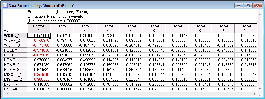
On the Factor rotation drop-down list, select Unrotated, and then click the Summary: Factor Loadings button to produce the Factor Loadings spreadsheet of loadings.
Remember that factors are extracted so that successive factors account for less and less variance (see the Introductory Overviews). Therefore, it is not surprising to see that the first factor shows most of the highest loadings. Also note that the sign of the factor loadings only counts insofar as variables with opposite loadings on the same factor relate to that factor in opposite ways. However, you could multiply all loadings in a column by -1 (i.e., reverse all signs), and the results would not be affected in any way.
Explained Variance for a given factor is the square of the loadings across the variables for the given factor.
Proportion of Total Variance is Explained Variance divided by the Total Variance in the data set.
In Factor Analysis, the analysis works on the correlation matrix or equivalently the standardized variables so that each variable is a variance of 1, thus, you can divide the explained variance by the total number of variables to get the proportion of total variance.
- Rotating the factor solution
- As described in the Introductory Overviews, the actual orientation of the factors in the factorial space is arbitrary, and all rotations of factors will reproduce the correlations equally well. This being the case, it seems natural to rotate the factor solution to yield a factor structure that is simplest to interpret; in fact, the formal term simple structure was coined and defined by Thurstone (1947) to basically describe the condition when factors are marked by high loadings for some variables, low loadings for others, and when there are few high cross-loadings, that is, few variables with substantial loadings on more than one factor. The most standard computational method of rotation to bring about simple structure is the varimax rotation (Kaiser, 1958); others that have been proposed are quartimax, biquartimax, and equamax (see Harman, 1967) and are implemented in Statistica.
- Specifying a rotation
- First, consider the number of factors that you want to rotate, that is, retain and interpret. It was previously decided that two is most likely the appropriate number of factors; however, based on the results of the Scree plot, it was also decided to look at the three-factor solution. We will start with three factors.
In the Factor Analysis Results dialog box, click the Cancel button to return to the Define Method of Factor Extraction dialog box, and change the Maximum no. of factors on the Quick tab from 10 to 3. Then click the OK button to continue with the analysis.
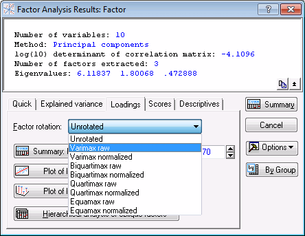
On the Factor Analysis Results dialog box - Loadings tab, on the Factor rotation drop-down list, select Varimax Raw to perform a varimax rotation.
Click the Summary: Factor loadings button to produce the Factor loadings spreadsheet.
- Reviewing the three-factor rotated solution
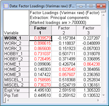
- In the Factor loadings spreadsheet, substantial loadings on the first factor appear for all but the home-related items. Factor 2 shows fairly substantial factor loadings for all but the work-related satisfaction items. Factor 3 only has one substantial loading for variable Home_1. The fact that only one variable shows a high loading on the third factor makes us wonder whether we cannot do just as well without it (the third factor).
- Reviewing the two-factor rotated solution
- Once again, click the Cancel button in the
Factor Analysis Results dialog box to return to the
Define Method of Factor Extraction dialog box. Change the Maximum no. of factors on the
Quick tab from 3 to 2 and click the OK button to continue to the Factor Analysis Results dialog box. Again select the
Loadings tab, and on the Factor rotation drop-down list, select Varimax raw. Click the Summary: Factor loadings button.
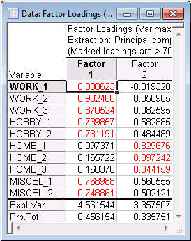
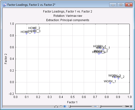
Factor 1 shows the highest loadings for the items pertaining to work-related satisfaction. The smallest loadings on that factor are for home-related satisfaction items. The other loadings fall in-between. Factor 2 shows the highest loadings for the home-related satisfaction items, lowest loadings for work-related satisfaction items, and loadings in-between for the other items.
- Interpreting the two-factor rotated solution
- Does this pattern lend itself to an easy interpretation? It looks like the two factors are best identified as the work satisfaction factor (Factor 1) and the home satisfaction factor (Factor 2). Satisfaction with hobbies and miscellaneous other aspects of life seem to be related to both factors. This pattern makes some sense in that satisfaction at work and at home may be independent from each other in this sample, but both contribute to leisure time (hobby) satisfaction and satisfaction with other aspects of life.
- Plot of the two-factor rotated solution
- Click the Plot of loadings, 2D button on the
Factor Analysis Results dialog box - Loadings tab to produce a scatterplot of the two factors. The graph simply shows the two loadings for each variable. Note that this scatterplot nicely illustrates the two independent factors and the 4 variables (Hobby_1, Hobby_2, Miscel_1, Miscel_2) with the cross-loadings.
Now we will see how well we can reproduce the observed correlation matrix from the two-factor solution.
- Reproduced and residual correlation matrix
- Select the
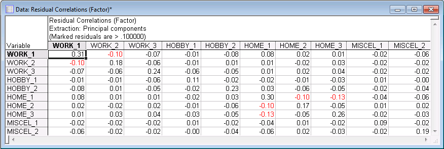
Explained variance tab, and click the Reproduced/residual corrs. button to produce two spreadsheets with the reproduced correlation matrix and the residual correlations (observed minus reproduced correlations).
The entries in the Residual Correlations spreadsheet can be interpreted as the "amount" of correlation that cannot be accounted for with the two factor solution. Of course, the diagonal elements in the matrix contain the standard deviation that cannot be accounted for, which is equal to the square root of one minus the respective communalities for two factors (remember that the communality of a variable is the variance that can be explained by the respective number of factors). If you review this matrix carefully you will see that there are virtually no residual correlations left that are greater than 0.1 or less than -0.1 (actually, a few are about of that magnitude). Added to that is the fact that the first two factors accounted for 79% of the total variance (see Cumulative % eigenvalues displayed in the Eigenvalues spreadsheet).
- The "secret" to the perfect example
- The example you have reviewed does indeed provide a nearly perfect two-factor solution. It accounts for most of the variance, allows for ready interpretation, and reproduces the correlation matrix with only minor disturbances (remaining residual correlations). Of course, nature rarely affords one such simplicity, and, indeed, this fictitious data set was generated via the normal random number generator accessible in the spreadsheet formulas. Specifically, two orthogonal (independent) factors were "planted" into the data, from which the correlations between variables were generated. The factor analysis example retrieved those two factors as intended (i.e., the work satisfaction factor and the home satisfaction factor); thus, had nature planted the two factors, you would have learned something about the underlying or latent structure of nature.
- Miscellaneous other results
- Before concluding this example, brief comments on some other results will be made.
- Communalities
- To view the communalities for the current solution, that is, current numbers of factors, click the Communalities button on the Factor Analysis Results dialog box - Explained Variance tab. Remember that the communality of a variable is the portion that can be reproduced from the respective number of factors; the rotation of the factor space has no bearing on the communalities. Very low communalities for one or two variables (out of many in the analysis) may indicate that those variables are not well accounted for by the respective factor model.
- Factor score coefficients
- The factor score coefficients can be used to compute factor scores. These coefficients represent the weights that are used when computing factor scores from the variables. The coefficient matrix itself is usually of little interest; however, factor scores are useful if one wants to perform further analyses on the factors. To view these coefficients, click the Factor score coefficients button on the Factor Analysis Results dialog box - Scores tab.
- Factor scores
- Factor scores (values) can be thought of as the actual values for each respondent on the underlying factors that you discovered. Click the Factor scores button on the Factor Analysis Results dialog box - Scores tab to compute factor scores. These scores can be saved via the Save factor scores button and used later in other data analyses.
- Final Comment
- Factor analysis is a not a simple procedure. Anyone who is routinely using factor analysis with many (e.g., 50 or more) variables has seen a wide variety of "pathological behaviors" such as negative eigenvalues, uninterpretable solutions, ill-conditioned matrices, and such adverse conditions. If you are interested in using factor analysis in order to detect structure or meaningful factors in large numbers of variables, it is recommended that you carefully study a textbook on the subject (such as Harman, 1968). Also, because many crucial decisions in factor analysis are by nature subjective (number of factors, rotational method, interpreting loadings), be prepared for the fact that experience is required before you feel comfortable making those judgments. The Factor Analysis module of STATISTICA was specifically designed to make it easy for you to switch interactively between different numbers of factors, rotations, etc., so that different solutions can be tried and compared.

