General Optimization Example

Overview

To use the General Optimization module, first you have to decide on the function that you need to optimize. The form of this function is problem specific, which can only be derived from the process model you want to optimize. This function must be defined in a Statistica Visual Basic (SVB) file and be accompanied by an active Statistica Spreadsheet that must contain all the necessary information for the optimization process. Following is a step-by-step example that highlights the minimum necessary requirements.

The first step is to define the mathematical function you want to optimize. For this example, the function consists of four variables, two continuous and two discrete, which are combined in the following form:

Function StatisticaGeneralOptimization(x() As Double) As Double
StatisticaGeneralOptimization = 0.5 + (x(1))*(x(1)) + (x(2))*(x(2)) + x(3) + x(4)
End Function

Next, prepare your optimization settings spreadsheet. For more details on how to create an optimization spreadsheet, see the Create new optimization spreadsheet option description in the Optimization Algorithm Tab topic. A copy of this spreadsheet, GeneralOptimizationSettings.sta, is located in the STATISTICA Examples > Datasets folder.

Data File

Open the GeneralOptimizationSettings.sta data file. Should you want to create your own spreadsheet, it must contain all the information necessary to the General Optimization analysis, such variable types (continuous or discrete); minimum, maximum, and starting values for the continuous variables; and number of unique values for the discrete variables.

Specifying the Analysis

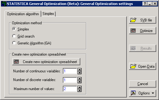
1. Select General Optimization from the Data Mining - Process Optimization submenu to display the STATISTICA General Optimization Startup Panel.
2. Click the SVB file button to locate and load the GeneralOptimizationSetting.svb file (located in the STATISTICA Examples > Macros > Analysis Examples folder). If the parsing of the SVB file and setting spreadsheet is successful, you are ready to start the optimization process. Before that, you can review the settings and change the value of the fields according to your optimization preferences.
3. You can change, for example, the minimum of the Simplex search for one or more continuous variables. To do so, select the Simplex option button on the Optimization algorithm tab. This displays the Simplex tab.
   
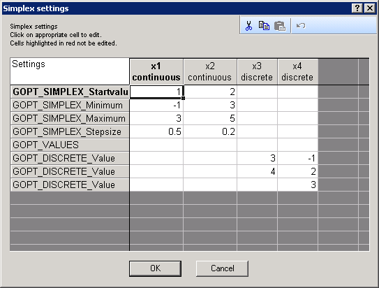
4. Select the Simplex tab and click the Change/review settings button. This displays a standard STATISTICA spreadsheet.
   
5. You can type in the desired value in the appropriate cell, and click OK. For this example, click Cancel to return to the STATISTICA General Optimization dialog box and use the original spreadsheet.
   Note: If any changes are made in the spreadsheet, they are displayed in the data grid area on the Simplex tab. Similarly, you can modify the settings for the Grid search and Genetic Algorithm by selecting the appropriate algorithm option on the Optimization algorithm tab.
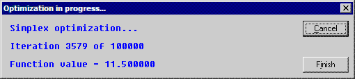
6. Click the Optimize button. This initiates the optimization algorithm. While computation is in progress, you can see a progress bar displaying information about the optimization process such as current function value and iteration number.
   
7. You can click Cancel to end the optimization and discard the results, and you can click Finish to end optimization and retain the results. Otherwise, the optimization continues until the stopping criterion is met. A set of outputs are displayed, which you can use to review and examine the optimization results. The results contain a settings spreadsheet particular to the algorithm used (Simplex in this case). Also displayed is a spreadsheet of final values of the variables that yield the minimum of the function defined in the SVB file. For this particular example, the optimized value of the variables are:
   
   Note: These optimal values are applicable to the particular settings (such as minimum and maximum) defined in the settings spreadsheet. If these conditions are changed, so may the optimal solution found by the algorithm. That is because by imposing a minimum and maximum on the variables range, you create what is known as a constrained optimization. Changing these constraints might yield different solutions.
8. In addition to these outputs, a spreadsheet of iteration is produced, which displays the function values per iteration. A graph representation of the spreadsheet can also be provided in the form of a two dimensional Statistica graph. Note that you can reprint the results of the optimization by clicking the Results button.