Example 5: Central Composite (Response Surface) Designs
Box, Hunter, and Hunter (1978, Chapter 15) report a study of the yield of a chemical process. The two factors of interest in that study are the setting of the temperature (variable Degrees) and the amount of Time that the chemical agents are allowed to react. Because you do not expect a simple linear relationship between these factors and the resultant yield, a response surface design is employed.
- Generating the Design
- Following are instructions to open the data file 2K-P.sta and start the Experimental Design (DOE) analysis from the ribbon bar and from the classic menus:
Ribbon bar. Select the Home tab. In the File group, click the Open arrow and from the menu, select Open Examples to display the Open a Statistica Data File dialog box. Double-click the Datasets folder, and open the 2K-P.sta data set. Then, select the Statistics tab, and in the Industrial Statistics group, click DOE to display the Design & Analysis of Experiments dialog box.
Classic menus. On the File menu, select Open Examples to display the Open a Statistica Data File dialog box. The 2K-P.sta data file is located in the Datasets folder. Then, on the Statistics - Industrial Statistics & Six Sigma submenu, select Experimental Design (DOE) to display the Design & Analysis of Experiments dialog box.
In the Startup Panel, on either the Quick tab or the Advanced tab, select Central composite, non-factorial, surface designs, and click the OK button to display the Design & Analysis of Central Composite (Response Surface) Experiments dialog box.
- Specifying the design
- The design described in Box, Hunter, and Hunter (1978) is a standard 2-factor central composite design. [Note that Study 1 reported by Hunter and Hunter, page 514, consists of a simple 22 factorial design with 3 center points; that design can be designed and analyzed via the 2(k-p) standard design (Box, Hunter, & Hunter) (two-level factorial designs) option in the
Startup Panel.]
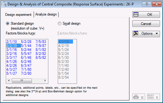
The distinction between Small designs and Standard designs pertains to the resolution of the cube portion of the design; for additional information concerning these designs; refer to the Introductory Overview.
For this study, we will select the standard 2-factor design in 10 runs and 2 blocks, that is, select Standard design 2/2/10.
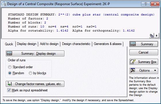
Click OK to display the Design of a Central Composite (Response Surface) Experiments dialog box.
- Design characteristic options
- The basic logic of central composite designs is described in the Introductory Overview. Most of the options in this dialog box are identical to those described for other designs in the previous examples. The
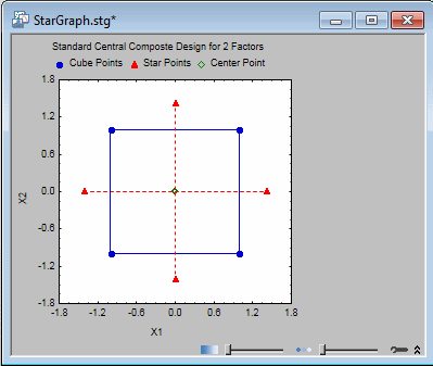
Design characteristic tab contains options that pertain to the factor settings for the star points of the design. Remember that the central composite design consists of a cube or square portion and a star portion, as shown in the following diagram.
The location of the star points determines whether the design is orthogonal (i.e., whether the factor effects are orthogonal) or rotatable. The concept of design rotatability is discussed in the Introductory Overview. In short, rotatability of the design refers to characteristics that the design can extract the same amount of information (i.e., make predictions with the same amount of precision) in all directions of the fitted surface. A design is orthogonal if the estimates of all terms in the second-order model are uncorrelated. In this blocked two-factor experiment, the same star-point setting a (alpha) will be computed either way.
Finalizing the Design
- Reviewing the standard design
- Let's first review the standard design. On the
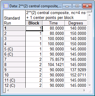
Quick tab, in the Order of runs group box, select the Standard order option button and click the Summary: Display design button to produce the spreadsheet.
These are the standard values for the coded factor levels (see Box, Hunter, and Hunter, 1978, page 519). However, because we later want to see the fitted response surface in terms of the original factor metric, let's select the factor settings now.
- Specifying the factor names and settings
- Return to the Design of a Central Composite (Response Surface) Experiments dialog box, and click the Change factor names, values, etc. button to display
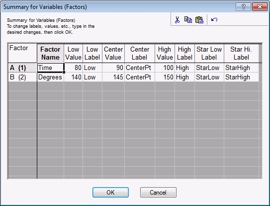
Summary for Variables (Factors) dialog box.
This dialog box is used to enter 1) the factor names, 2) their high, low, and center settings, 3) the text labels for those settings, and 4) the text labels for axial or star points. For this experiment, we will not enter text labels; however, enter the factor names and values for the factor low, center, and high settings as follows.
Click the OK button.
- Adding center points
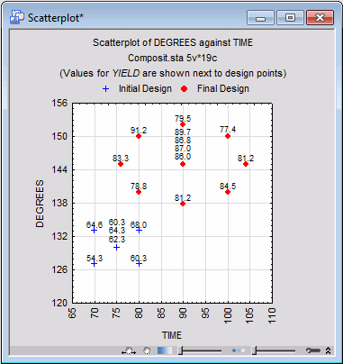
- Box, Hunter, and Hunter (1978, page 519) added to the standard design 1 center point in each block (i.e., 2 points were added, one in the cube portion and one in the star portion of the design). Select the Add to design tab, and enter a 1 in the Number of center points (per block) box.
- Saving the final design
- Return to the
Quick tab, and click the Summary: Display design button again to produce the spreadsheet with the final design.
Now the axial star points are no longer displayed in their coded form (1.4142), but in the metric of the factors (note that the axial star points are computed relative to the center points, i.e., they are equidistant from the center points as defined by the user via the Change factor names, values, etc. button).
Save this design via File - Save As. Close the dialog box and all displayed spreadsheets/workbooks.
- Analyzing the Design
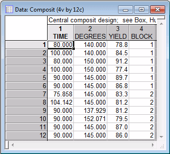
- The data file Composit.sta contains the results for the experiment (see Box, Hunter, and Hunter, 1978). Open this data file.
- Specifying the design
- In the Experimental Design Startup Panel, select Central composite, non-factorial, surface designs and click OK.
In the Design & Analysis of Central Composite (Response Surface) Experiments dialog box, select the Analyze design tab.
Click the Variables button, and select Yield as the Dependent variable, Time and Degrees as the Indep. (factors), and Block as the Blocking variable. (You may need to clear the Show appropriate variables only check box in the variable selection dialog box.)
Click OK in the variable selection dialog box. A message will be displayed concerning text variables. Click the Continue with current selection button.
- Rescaling of factors
- If you are using standard central composite designs, Statistica can automatically determine how to rescale the factor values from the respective low and high values [as with other designs, the program will perform the ANOVA on the scaled (±1 and a) factor values; although the coefficients for the untransformed variables can also be computed].
However, if your design is not a standard central composite design, you should select the User-defined high/low factor values option button, and Statistica will prompt you to enter the low and high settings for each factor. Thus, any response surface design can be analyzed.
Because the current design is a standard central composite design, click OK to proceed.
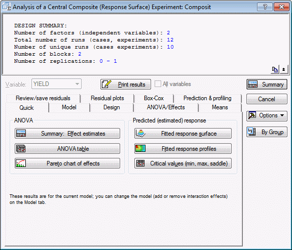
The Analysis of a Central Composite (Response Surface) Experiment dialog box contains essentially the same options as already discussed in previous examples (e.g., see Example 1.1).
Analysis of Variance
- Pure error and lack of fit
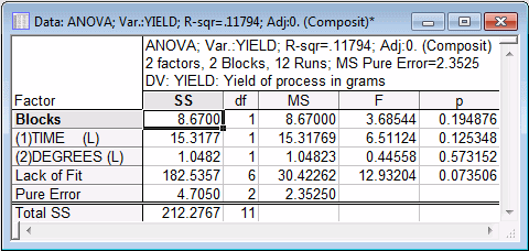
- Because the design includes 1 extra center point per block, we can estimate the pure error, and test for overall lack of fit. As discussed in the Introductory Overview, when at least some points (preferably center points) are replicated, we can estimate the random measurement variability (reliability) for the dependent variable from the variability of the measurements taken at those identical points in the design. This enables you to test the residual variability (which is not accounted for by the factors and their interactions) for statistical significance. If the test is statistically significant, it is an indication of the inadequacy or lack of fit of the current model.
- ANOVA table for linear main effects model
- To illustrate this test, let's begin by testing the simplest model.
Select the Model tab. In the Include in model group box, select the Linear main effects only option button. In the ANOVA error term group box, select the Pure error option button.
Then select the Quick tab (or ANOVA/Effects tab) and click the ANOVA table button.
None of the linear main effects approaches statistical significance; however, the Lack of fit test is marginally significant (p<.10), suggesting, that the simple linear main-effects-only model is too simple.
- ANOVA table for second-order model
- Now, create the ANOVA table for the full second-order model. Click on the
Model tab, and select the Lin/quad main eff.+2-ways option button. Then, click the ANOVA table button again.
It appears that the interaction effect, as well as the quadratic effects are statistically significant (p<.05) or marginally significant (p<.10).
- Parameter Estimates and Coefficients
- Next, we will review the ANOVA parameter estimates and coefficients. Select the
Quick tab (or
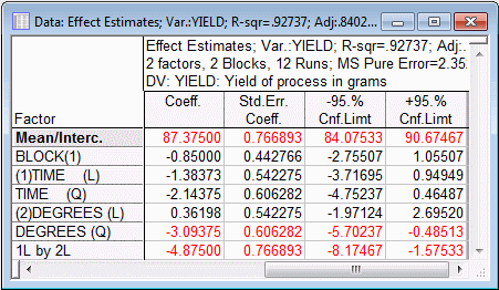
ANOVA/Effects tab) and click the Summary: Effect estimates button.
The last four columns of the spreadsheet are shown above, including the coefficient estimates for the linear prediction equation for the recoded factor values. Thus, you could use these values to predict values for Yield as:
where ypred. stands for the predicted Yield values, and x1 and x2 stand for the recoded (±1, 0, or a) factor values (Time and Degrees, respectively). Note that we have ignored the Block effect in the equation above, since that effect was not significant. Also, the Block coefficient would be applied to a "dummy-variable" or coded variable that reflects the assignment of a case to a block; for prediction purposes this value is best set to 0 (zero).
- Regression coefficients
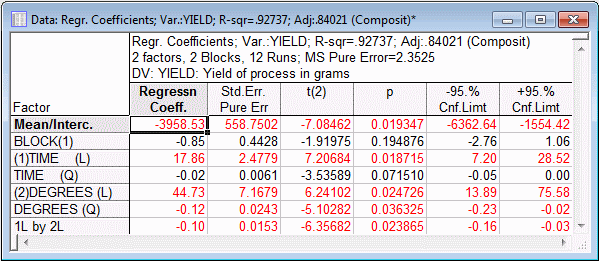
- If you want to use untransformed factor values in the prediction equation, use the Regression coefficients instead. Select the ANOVA/Effects tab, and click the Regression coefficients button.
- Predicting values for the dependent variable
- There is a designated option available for predicting values of the dependent variable, based on user-defined factor values.
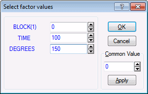
Select the Prediction & profiling tab. Click the Predict dependent variable values button. A message will be displayed concerning blocking. See Main Effects and Interactions for Central Composite Experiments for more information. Click OK in the message. In the Select factor values dialog box, enter 0 for Block(1), 100 for Time, and 150 for Degrees.
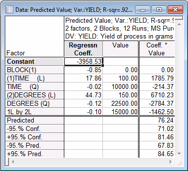
Thus, we will predict the Yield of the chemical process, based on the current model, for the factor settings 100 minutes and 150° Celsius. Click OK to review the results.
The predicted value for Yield is equal to 76.24. Note that the confidence intervals are computed from the current estimate of Error for the model, that is, as displayed in the ANOVA spreadsheet.
- Response Surface and Contours
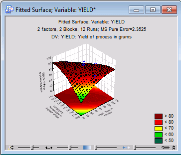
- The most common way to summarize the results of a central composite design experiment is in the form of a response surface or via response contours.
On the Prediction & profiling tab (or the Quick tab), click the Surface plot (fitted response) button. In the Select factor values dialog box, accept the default value for the Block variable (0) and click OK.
Note: you can use the Interactive Graphics Controls at the bottom of the graph window to adjust the plot areas transparency and to scroll and pan in order to interactively scale the graph.Next, click the Contour plot (fitted response) button.
- A Note on the Method of Steepest Ascent
- In practice, the response surface usually exhibits curvature near its maximum; in the regions far away from the maximum, curvature is often negligible. Therefore, in the early stages of the search for the optimum settings of levels for factors, we sometimes run the cube portion of the design only and examine the resulting contour plot (here, with no two-way interaction, i.e., on the
Model tab select Linear main effects only).
For example, for the chemical Yield example discussed above, Box, Hunter, and Hunter (1978, page 514) ran, as a first study, a 22 factorial design, enhanced with 3 center points, and fitted the linear main-effects model shown above.
If we now drew a line perpendicular to the contours, this line would represent the path of steepest ascent toward the maximum of the function.
The coefficients estimated for that model will tell you how to proportionally change the levels of the factors in the design to follow this path. Continuous curvature checks during this stage of the search will inform you when you approach the maximum of the function.
See also, Experimental Design Index.

