GLZ Introductory Overview - Computational Approach
To summarize the basic ideas, the generalized linear model differs from the general linear model (of which, for example, multiple regression is a special case) in two major respects: First, the distribution of the dependent or response variable can be (explicitly) non-normal, and does not have to be continuous, i.e., it can be binomial, multinomial, or ordinal multinomial (i.e., contain information on ranks only); second, the dependent variable values are predicted from a linear combination of predictor variables, which are "connected" to the dependent variable via a link function. The general linear model for a single dependent variable can be considered a special case of the generalized linear model: In the general linear model the dependent variable values are expected to follow the normal distribution, and the link function is a simple identity function (i.e., the linear combination of values for the predictor variables is not transformed).
To illustrate, in the general linear model a response variable Y is linearly associated with values on the X variables by
Y = b0 + b1X1 + b2X2 + ... + bkXk + e
(where e stands for the error variability that cannot be accounted for by the predictors; note that the expected value of e is assumed to be 0), while the relationship in the generalized linear model is assumed to be
Y = g (b0 + b1X1 + b2X2 + ... + bkXk) + e
where e is the error, and g(...) is a function. Formally, the inverse function of g(...), say f(...), is called the link function; so that:
f ( muy) = b0 + b1X1 + b2X2 + ... + bkXk
where muy stands for the expected value of y.
- Link functions and distributions
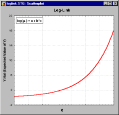
- Various link functions (see McCullagh and Nelder, 1989) can be chosen, depending on the assumed distribution of the y variable values:
Normal, Gamma, Inverse normal, and Poisson distributions:
Identity link: f(z) = z
Binomial, and Ordinal Multinomial distributions:
Logit link: f(z)=log(z/(1-z))
Probit link: f(z)=invnorm(z) where invnorm is the inverse of the standard normal cumulative distribution function (see Distributions and their functions).
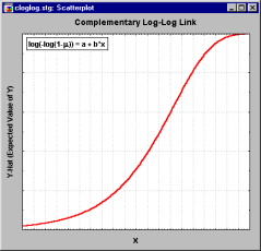
Complementary log-log link: f(z)=log(-log(1-z))
Multinomial distribution:
Generalized logit link: f(z1|z2, ..., zc)=log(x1/(1-z1-...-zc)) where the model has c+1 categories.
- Estimation in the generalized linear model
- The values of the parameters (b0 through bk and the scale parameter) in the generalized linear model are obtained by maximum likelihood (ML) estimation, which requires iterative computational procedures. There are many iterative methods for ML estimation in the generalized linear model, of which the Newton-Raphson and Fisher-Scoring methods are among the most efficient and widely used (see Dobson, 1990). The Fisher-scoring (or iterative re-weighted least squares) method in particular provides a unified algorithm for all generalized linear models, as well as providing the expected variance-covariance matrix of parameter estimates as a byproduct of its computations. STATISTICA uses the Fisher-Scoring method.
- Statistical significance testing
- Tests for the significance of the effects in the model can be performed via the Wald statistic, the likelihood ratio (LR), or score statistic. Detailed descriptions of these tests can be found in McCullagh and Nelder (1989). The Wald statistic (e.g., see Dobson, 1990), which is computed as the generalized inner product of the parameter estimates with the respective variance-covariance matrix, is an easily computed, efficient statistic for testing the significance of effects. The score statistic is obtained from the generalized inner product of the score vector with the Hessian matrix (the matrix of the second-order partial derivatives of the maximum likelihood parameter estimates). The likelihood ratio (LR) test requires the greatest computational effort (another iterative estimation procedure) and is thus not as fast as the first two methods; however, the LR test provides the most asymptotically efficient test known. For details concerning these different test statistics, see Agresti(1996), McCullagh and Nelder(1989), and Dobson(1990).
- Diagnostics in the generalized linear model
- The two basic types of residuals are the so-called Pearson residuals and deviance residuals. Pearson residuals are based on the difference between observed responses and the predicted values; deviance residuals are based on the contribution of the observed responses to the log-likelihood statistic. In addition, leverage scores, studentized residuals, generalized Cook's D, and other observational statistics (statistics based on individual observations) can be computed. For a description and discussion of these statistics, see Hosmer and Lemeshow(1989).


