Example: Model Profiler in DOE
Ribbon bar. Select the Home tab. In the File group, click the Open arrow and select Open Examples to display the Open a STATISTICA Data File dialog box. The data file is located in the Datasets folder. Then, select the Statistics tab. In the Industrial Statistics group, click DOE to display the Design & Analysis of Experiments Startup Panel.
Classic menus. From the File menu, select Open Examples to display the Open a STATISTICA Data File dialog box. The data file is located in the Datasets folder. Then, from the Statistics - Industrial Statistics & Six Sigma submenu, select Experimental Design (DOE) to display the Design & Analysis of Experiments Startup Panel.
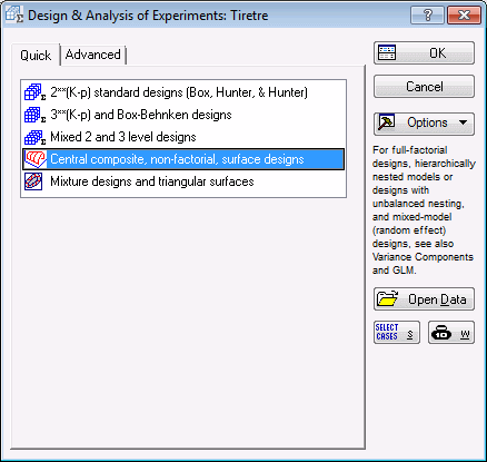
On the Quick tab of the Startup Panel, select Central composite, non-factorial, surface designs.
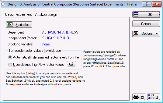
Click the OK button to display the Design & Analysis of Central Composite (Response Surface) Experiments dialog box.
Select the Analyze design tab.
Click the Variables button to display the variable selection dialog box. Select 1-4 as Dependent and 5-7 as Indep. (factors). Click OK.
In the Design & Analysis of Central Composite (Response Surface) Experiments dialog box, click OK.
In the Analysis of a Central Composite (Response Surface) Experiment dialog box, select the Model tab. Ensure that the Lin/quad main eff. +2-ways option button is selected in the Include in model group box.
Click the Model Profiler button (located in the lower-left corner of the tab).
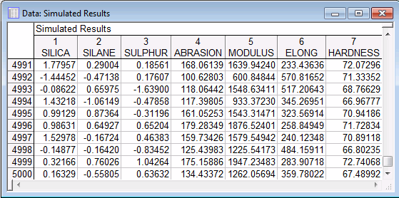
By default, STATISTICA automatically performs 5,000 simulations and detects the most appropriate distribution for each of the predictor variables. A data file is generated with results from the 5,000 simulations,
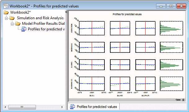
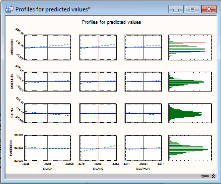
and a workbook is generated with profiles for predicted values.
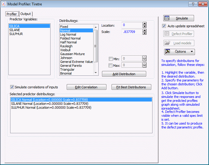
In the Model Profiler dialog box, in addition to the default, you can either: 1) automatically fit the best distribution to each of the predictor variables, or 2) manually assign a distribution to a predictor variable with custom parameters if desired.
To manually assign a distribution with custom parameters: 1) select a specific predictor from the Predictor Variables list, 2) select the appropriate distribution from the Distributions list and set the specific parameters as appropriate, and then 3) click the Add Distribution button. This will assign the distribution, with custom parameters if specified, to the predictor selected. The settings can be verified in the Selected predictor distributions box. After modifying any of the settings for the predictor variables, you can again automatically fit the best distributions to each of the predictor variables by clicking the Fit Best Distributions button.
In the above example, the Fit Best Distributions button was clicked in the Model Profiler.
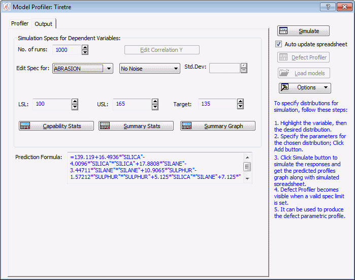
Now, select the Output tab.
Change No. of runs to 1000. From the Edit Spec for list, select ABRASION, and enter 100 for LSL, 165 for USL and 135 for Target.
STATISTICA will automatically store these settings.
Next, from the Edit Spec for list, select HARDNESS, and enter 54 for LSL, 90 for USL and 69.8 for TARGET.
Click the Simulate button.
Two .sta files and one workbook are produced. One .sta file includes the simulated results.
One .sta file includes the defect rate for ABRASION and HARDNESS.
The Workbook contains profiles for predicted values.
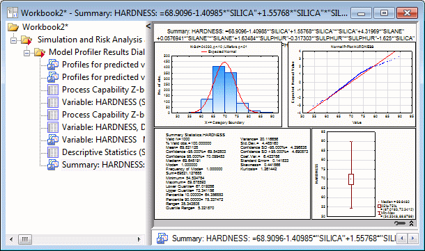
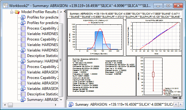
In the Model Profiler, verify that HARDNESS is specified in the Edit Spec for list. Click the Capability Stats button, the Summary Stats button, and the Summary Graph button. Review the results for HARDNESS in the workbook.
Now, in the Model Profiler, in the Edit Spec for list, select ABRASION. Click the Capability Stats, Summary Stats, and Summary Graph buttons. Review the results for ABRASION in the workbook.

