Monte Carlo Example 3: Bootstrapping

Bootstrapping (Efron, 1982) is a general technique for estimating sampling distributions. If N independent observations from a population are available, bootstrapping simulates the sampling distribution of any statistic by treating the observed data as if it were the entire (discrete) statistical population under study. Suppose, for example, you want to estimate the sampling distribution of the correlation coefficient in order to set a confidence interval for the correlation between two variables. You only have a sample of size 200 from the relevant population. If the population variables can be reasonably assumed to have a bivariate normal distribution, you could use the well-known procedures available in virtually any textbook. However, suppose your data depart seriously from a bivariate normal distribution, and, moreover, you do not have access to more general results (e.g., Steiger and Hakstian, 1982) on the distribution of the correlation coefficient with non-normal data. In this case, setting up a confidence interval using the standard "normal theory" procedures might yield serious errors. How might you proceed in this case?

The way bootstrapping works is as follows. On each replication, a random sample of size N is selected, with replacement, from the available data. The statistic of interest is calculated on this "bootstrapped subsample," and recorded. The process is repeated for some reasonable number of replications. Finally, the distribution of all the bootstrapped statistics is tabulated. This distribution furnishes an approximation to the actual sampling distribution of the statistic. Note again that, in effect, bootstrapping assumes that the population distribution can be approximated by a discrete distribution identical to that manifested in your sample.

SEPATH's Monte Carlo module has a bootstrapping facility built into it. This facility takes random samples (with replacement) of size N from the current data file, fits the current model to that "bootstrapped subsample," and stores the results. You can use this facility to estimate the sampling distribution of model parameters or to perform Monte Carlo simulations of sampling from discrete multivariate distributions.

In this case, bootstrapping will be employed to estimate the standard error of a correlation coefficient from a non-normal multivariate population.

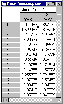
The data file Bootsamp.sta contains a sample of 200 observations on two variables. Open this data file, and start the Structural Equation Modeling module:

Ribbon bar. Select the Home tab. In the File group, click the Open arrow and select Open Examples to display the Open a STATISTICA Data File dialog box. Open the Datasets folder. Open the data file, which is located in the SEPATH folder. Then, select the Statistics tab. In the Advanced/Multivariate group, click Advanced Models and from the menu, select Structural Equation to display the Structural Equation Model Startup Panel.

Classic menus. From the File menu, select Open Examples to display the Open a STATISTICA Data File dialog box. Open the Datasets folder. Open the data file, which is located in the SEPATH  folder. Then, from the Statistics - Advanced Linear/Nonlinear Models submenu, select Structural Equation Modeling to display the Structural Equation Model Startup Panel.

For this example, we will use model file 2var.cmd. This "fully saturated" model simply estimates the population correlation matrix.

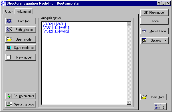
In the Structural Equation Modeling Startup Panel, select the Advanced tab and click the Open model button. In the Open Model Syntax dialog box, select the model file 2var.cmd and click the Open button.

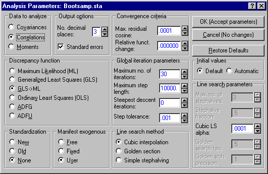
Now, fit this model to the observed data. On the Structural Equation Modeling Startup Panel - Advanced tab, click the Set parameters button to display the Analysis Parameters dialog box.

In the Data to analyze group box, select the Correlations option button. Ensure that the default Discrepancy function, GLS->ML, is selected, and then click the OK (Accept parameters) button.

When you return to the Startup Panel, begin estimation by clicking OK (Run model). Since the model is fully saturated, there are no degrees of freedom, and you will quickly converge to a discrepancy function that is essentially zero. In the Structural Equation Modeling Results dialog - Quick tab, click the Model summary button. You will see the correlation parameter estimated at .499, and its standard error at .053. Can this latter estimate be trusted?

There is strong evidence that the population distribution is not multivariate normal in this case. The variables have high kurtosis. Consequently, the estimated standard error obtained under the assumption of multivariate normality may be seriously biased.

In this case, there are two options. One is to employ Asymptotically Distribution Free (ADF) estimation procedures. Another is to employ bootstrapping.  

We will use the latter option and bootstrap an estimate of the sampling variability of the correlation coefficient, using the Monte Carlo module's bootstrapping function. Open the Bootsamp.sta data file and launch the Structural Equation Modeling module. On the Advanced tab, open the model file 2var.cmd.

Click the Set parameters button to display the Analysis Parameters dialog box, and choose Correlations as the Data to analyze. Click OK (Accept parameters) to return to the Startup Panel.

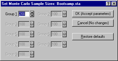
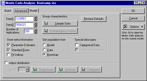
Click the Monte Carlo button on the Startup Panel to display the Monte Carlo Analysis dialog box. Choose Bootstrap as the option under Get population from. Click the Sample Sizes button to display the Set Monte Carlo Sample Sizes dialog box, and set the sample size to 200.

Click the OK (Accept parameters) button to return to the Monte Carlo Analysis dialog box, enter 200 as the Number of replications, and select the Parameter Estimates and Standard Errors check boxes under Store extra information.  

Click the OK button to start the Monte Carlo study. When the bootstrap data have been gathered, click the Summary: Display overall results button on the Monte Carlo Results dialog box to display a spreadsheet containing the results of the Monte Carlo analysis. While the spreadsheet is the active window, select Save As from the File menu. Enter Boot1.sta as the file name, and save the file.  

The bootstrap data have now been saved as a STATISTICA data file. To construct an empirical estimate of the characteristics of the sampling distribution of the correlation coefficient, open the Boot1.sta data file (or, if it is still open, select Input Spreadsheet from the Data menu to specify Boot1.sta as the input data file), and call up the Basic Statistics and Tables module.

Begin by constructing a histogram of the variable PAR_1, which contains the estimated correlation coefficients. To construct the histogram, select Frequency tables from the Basic Statistics and Tables Startup Panel to display the Frequency Tables dialog box.

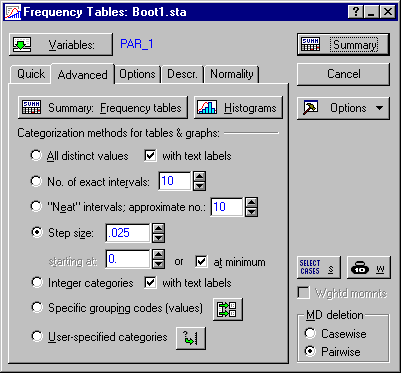
Click the Variables button, select PAR_1 as the variable, and click OK to return to the Frequency Tables dialog box. Under Categorization method for tables and graphs, select the Step size option button, enter .025 in the adjacent box, and select the at minimum check box adjacent to the starting at box.

Click the Histograms button to produce a graph as shown below. This histogram provides an estimate of the sampling distribution of the correlation coefficient, based on your data. As you can see, the distribution of the sample correlation coefficient follows a normal distribution very closely.

Next, calculate the standard deviation of the parameter estimates to obtain an estimate of the standard error of the correlation coefficient.

From the Basic Statistics and Tables Startup Panel, select Descriptive Statistics and compute Summary: Descriptive Statistics for variable PAR_1. You should obtain the following:

The standard deviation of the bootstrap value estimates the standard error of the correlation coefficient as .0581, substantially larger than the estimate provided by the maximum likelihood estimation procedure.  

We can compare this estimate with one obtained via ADF estimation. Open Bootsamp.sta, return to the SEPATH module, and open 2Var.cmd again; then estimate the model with ADFU selected as the Discrepancy function, and Correlations as the Data to analyze.

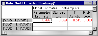
You will obtain an estimated standard error of .059 for the correlation parameter.

Actually, the data in Bootsamp.sta were generated by the SEPATH Monte Carlo module. The population distribution is multivariate nonnormal. The variables were transformed using the Vale-Maurelli procedure to have population skewnesses of 0, but population kurtoses of 15 each. By running a large Monte Carlo study (using Structural Equation Modeling), we determined the actual standard error of the correlation coefficient to be .069 in this case. You can see that the ADF procedure provided the most accurate estimate of the standard error, the bootstrap a somewhat less accurate estimate, and the maximum likelihood procedure the worst estimate.  

The ADF and bootstrapping estimates might have been more accurate, but in this case the sample kurtoses for the data in Bootsamp.sta were rather substantial underestimates of the actual population values of 15.