Example 7: Constructing a Confidence Interval on the Noncentrality Parameter
In Example 6, we discuss how to test a hypothesis about the noncentrality parameter of a noncentral F distribution. We mention that such a hypothesis test has a number of practical applications, because the noncentrality parameter can be related to a number of meaningful statistical quantities. In this example, we show how to use the Noncentral F Probability Calculator to construct a confidence interval on the noncentrality parameter of the noncentral F distribution. Such confidence intervals can be used to construct confidence intervals on a number of interesting quantities. For example, in the context of ANOVA, we can construct exact confidence intervals on ω2, the proportion of variance accounted for by the treatment effects.
For a discussion of the rationale behind noncentrality interval estimation, consult the article by Steiger and Fouladi (1997). The method itself is quite simple.
Suppose you observe a value X on a noncentral F variate. You know the degrees of freedom, and you would like to construct a 1 - α confidence interval on the noncentrality parameter, δ. For example, what is frequently referred to as a "90% confidence interval" is a .90 confidence interval, with α = .05.
To construct the 1 - α confidence interval, proceed as follows:
- Find the cumulative probability for the observed value, x, with the known degrees of freedom, and a δ of zero. If that cumulative probability is less than or equal to 1 - α/2, then the lower confidence limit for the noncentrality parameter is zero. Otherwise, you compute the lower confidence limit by solving for the value of the noncentrality parameter, δ, for which the observed x has cumulative probability 1 - α/2.
- If the lower limit is not above zero, then proceed to step 3. Otherwise, again consider the cumulative probability for the observed value, x, with the known degrees of freedom, and a δ of zero. If that cumulative probability is less than or equal to α/2, then the upper confidence limit for the noncentrality parameter is zero. Otherwise, proceed to step 3.
- Compute the upper confidence limit by solving for the value of the noncentrality parameter, δ, for which observed value x has cumulative probability α/2.
Note also that there is a direct correspondence between this confidence interval and a hypothesis test on the noncentrality parameter. For example, if you are testing a 1-tailed hypothesis that δ <= c against the alternative that δ > c, the hypothesis test at the α significance level will reject if and only if the 1 - 2α confidence interval does not include c within its limits. Similarly, a 2-tailed hypothesis at the α significance level that δ = c tested against the alternative that δ ≠ c will be rejected if and only if the 1 - α confidence interval excludes c.
So, for example, one can actually perform a 1-tailed hypothesis test that δ <= 2 against the alternative that δ > 2 at the .01 level by examining whether the .98 (i.e., 98%) confidence interval does not include 2 within its limits.
As an example of this kind of confidence interval, suppose we use the same values employed in Example 6. A value of F with 3 and 36 degrees of freedom has been observed to be 7.35. We will now use this information to construct a 98% confidence interval on δ, using the steps described above. (Note that, in what follows α = .01, and that the confidence interval is a .98 confidence interval, so that the α for the confidence interval will be .02.
Ribbon bar. Select the Statistics tab. In the Advanced/Multivariate group, click Power Analysis to display the Power Analysis and Interval Estimation Startup Panel.
Classic menus. From the Statistics menu, select Power Analysis to display the Power Analysis and Interval Estimation Startup Panel.
In the Startup Panel, select Probability Distributions and Noncentral F Distribution.
Now, click the OK button to display the Noncentral F Probability Calculator dialog box.
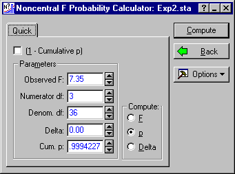
To perform the first step of the computation, enter 7.35 in the Observed F box, 3 in the Numerator df box, and 36 in the Denom. df box. Make sure that p is selected under Compute, and then click the Compute button to obtain the cumulative probability. The result will be .9994227. Since this is above 1 - .02/2 (.99), we know that the lower confidence bound will be above zero.
Next, solve for the value of Delta that will place the Observed F value at the 1 - α/2 cumulative probability point. Enter .99 in the Cum. p box, and select the Delta option button under Compute to make δ the item to compute. Click the Compute button, and Statistica will obtain a value of Delta for which 7.35 has a cumulative probability of precisely .99.
The lower limit of the 98% confidence interval for δ is 2.66728. Since the lower limit is above zero, we proceed to step 3 of the general procedure, and compute the value of Delta for which 7.35 has a cumulative probability of precisely .01. Simply enter .01 in the Cum. p box, and click the Compute button.
The upper confidence limit for δ is 51.38733. Consequently, a 98% confidence interval for δ ranges from 2.66728 to 51.38733. This confidence interval does not include two, so we can also determine immediately that a 1-tailed hypothesis that δ <= would be rejected at the .01 level.
See also, Power Analysis - Index.


