Example 1.3: Analyzing a Botched 2(7-4) Fractional Factorial Design
In Example 1.1: Designing and Analyzing a 2(7-4) Fractional Factorial Design, we studied the effect of 7 different factors on the speed with which a bicyclist can climb a hill (see also, Box, Hunter, and Hunter, 1978). Let's suppose that on one of the runs for this hypothetical experiment, the gear was incorrectly adjusted to the second level rather than the first (lowest) level so that the run was no longer consistent with the original design. Such imprecise settings will alter the properties (confounding, resolution) of the experiment; however, unless the experimental runs are grossly mismatched (different from the desired values), valid and meaningful analyses can still be conducted. These so-called botched designs can still be analyzed correctly in STATISTICA Experimental Design
- Botching the Experiment
- To begin, open the example data file Cycling.sta.
Ribbon bar. Select the Home tab. In the File group, on the Open menu, select Open Examples to display the Open a STATISTICA Data File dialog box. Double-click the Datasets folder, and then open the data set.
Classic menus. On the File menu, click Open Examples to display the Open a STATISTICA Data File dialog box. The data file is located in the Datasets folder.
The (fictitious) results in this data file were reported by Box, Hunter, and Hunter (1978, page 391).
Shown here are the original settings for the factors; note that text values (e.g., Up, Down) were also entered to identify the respective settings. You can toggle between text and numeric values in the data file by clicking the Show/hide text labels button.
Let's assume that for the second run, the gear was not actually shifted to the low position; instead, it was shifted to the second lowest position. To make this modification, enter a -0.8 in the second case of the variable GEAR. The data will now look as shown below.
- Specifying the design
- Select the Experimental Design (DOE) analysis.
Ribbon bar. Select the Statistics tab, and in the Industrial Statistics group, click DOE to display the Design & Analysis of Experiments Startup Panel.
Classic menus. From the Statistics - Industrial Statistics & Six Sigma submenu, select Experimental Design (DOE) to display the Design & Analysis of Experiments Startup Panel.
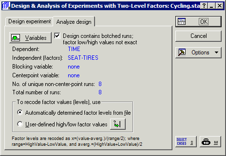
Then select 2**(k-p) standard designs (Box, Hunter, and Hunter) from the Startup Panel and click the OK button. In the Design & Analysis of Experiments with Two-Level Factors dialog, click on the Analyze design tab, and select the Design contains botched runs; factor low/high values not exact check box. Next, click the Variables button to select the Dependent and Indep. (factors). The dependent variable in this case is variable Time, which contains the times that the person required to cycle up the hill; variables Seat through Tires are the independent variables because they contain the codes (+1,-1) that uniquely identify to which group in the design the respective case belongs. For this example, we will let STATISTICA determine factor levels from the data file itself, so you do not need to make changes to the To recode factor values (levels), use options. The dialog will look like this.
- Reviewing results
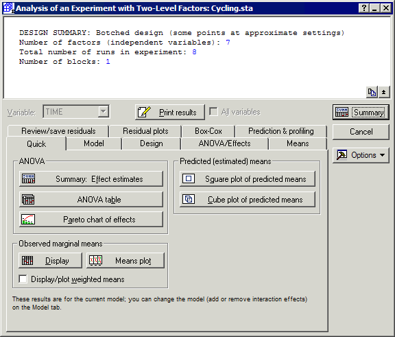
- Now, click the OK button, and the Analysis of an Experiment with Two-Level Factors dialog will be displayed.
- Main effects
- Now click on the
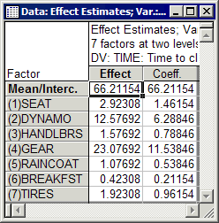
ANOVA/Effects tab and click the Summary: Effect estimates button to display this spreadsheet with the effect estimates.
As with Example 1.1, STATISTICA will fit a simple main effects model, without interactions. Remember that our initial design is of resolution III (3); hence, the two-way interactions are confounded with the main effects, and they cannot be estimated from this design. The first numeric column of the spreadsheet shown above contains the Effect estimates. These parameter estimates can be interpreted as deviations of the mean of the negative settings from the mean of the positive settings for the respective factors. Recall that even though our design is botched (i.e., for one run, the seat setting was at -.8 instead of -1, the scaling was still for a minimum of -1 and a maximum of 1. So, for example, the Effect column gives us the estimate of what happens when the factor goes from its low value to its high value. When the seat position went from down (-1) to up (+1), the time to climb the hill increased by an average of 2.92 seconds. The second numeric column contains the effect Coefficients. These are the coefficients that could be used for the prediction of climb-time for new factor settings, via the linear equation:
ypred. = b0 + b1*x1 + ... + b7*x7
where ypred. stands for the predicted climb-time, x1 through x7 stand for the settings of the factors (1 through 7), b1 through b7 are the respective coefficients, and b0 stands for the intercept or mean.
See also, Experimental Design Index.