Example 2: Discriminant-Based Univariate Splits for Categorical and Ordered Predictors
This example illustrates an analysis of the Boston housing data (Harrison & Rubinfeld, 1978) that was reported by Lim, Loh, and Shih (1997). Median prices of housing tracts are classified as Low, Medium, or High on the dependent variable Price. There is 1 categorical predictor, Cat1, and 12 ordered predictors, Ord1 through Ord12. A duplicate of the learning sample is used as a test sample. The sample identifier variable is Sample and contains codes of 1 for Learning and 2 for Test. The complete data set containing a total of 1012 cases is available in the example data file Boston2.sta. Open this data file via the File - Open Examples menu; it is in the Datasets folder. Part of this data file is shown below.
Specifying the analysis
With two exceptions (i.e., the specifications for Priors and V-fold for cross-validation), we will use the default analysis options in the Classification Trees module. Select Classification Trees from the Statistics - Multivariate Exploratory Techniques menu to display the Classification Trees Startup Panel. On the Quick tab, select the Variables button to display the standard variable selection dialog. Here, select Price as the Dependent variable, Cat1 as a Categorical preds., Ord1 through Ord12 as Ordered predictors, Sample as the Sample identifier variable, and then click the OK button. Next, click on the Methods tab and select the Equal option button under Prior probabilities. Then, click on the Sampling options tab and enter 10 in the V-fold cross-validation, v value field. Finally, click the OK button on the Classification Trees Startup Panel to first briefly display the Parameter Estimation dialog (from which you can monitor the progress of the classification tree computations) and then the Classification Trees Results dialog when the computations are completed.
Reviewing the results
Click on the Tree structure tab and then click the Tree sequence button to display the spreadsheet shown below.
As the spreadsheet shows, the selected tree (Tree number 29, denoted with a *) has a CV cost of .2621 with a Std. error of .0194, costs for the learning sample, labeled as Resub. (Resubstitution) cost, of .2410, and a "smoothed" Node complexity value of .0043 The minimum CV cost trees (Tree numbers 23 and 24) have CV costs of .2482 with Std. errors of .0191, and the selected tree is the simplest tree with a CV cost not exceeding .2482 + .0191 = .2673, using the default 1.0 Standard error rule (see the Stopping options tab).
The sequence of Resubstitution and CV costs can be graphically displayed by clicking the Cost sequence button to produce the graph shown below.
Next, on the Cross-validation tab, click the Misclassification matrix button under Test sample to display the spreadsheet shown below.
This spreadsheet shows the number of cases in the test sample in each observed class misclassified as each of the other two classes. The CV cost and the standard deviation of the CV cost (s.d. CV cost) based on the test sample misclassifications are displayed in the header area of the spreadsheet. Note that because the test sample is a duplicate of the learning sample, the CV cost for the test sample is the same as the Resubstitution cost for the learning sample shown in the previous spreadsheet. Note also that predicted classes and terminal node assignments for each case in the test sample can be displayed on a spreadsheet by clicking the Predicted cases button under Test sample.
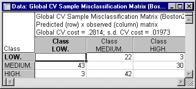
Now, on the Cross-validation tab, enter 10 in the v-fold for GCV field and then click the Perform global CV button to display the Global cross-validation dialog. Click the Global CV misclassification matrix button, which will first open the Global CV Parameter Estimation dialog from which you can monitor the progress of the global cross-validation computations. Upon completion of the cross-validation procedure, the Global CV Sample Misclassification Matrix spreadsheet is displayed.
The Global CV cost and its standard deviation (s.d. CV cost) are fairly similar to the CV cost and its Standard error for the selected tree (Tree number 29, see above), indicating that the "automatic" tree selection procedure fairly consistently selects a tree with close to the minimum estimated cost.
In this example the selected "right-sized" tree has 8 terminal nodes, 7 splits, and 14 branches (see the Classification tree plot button on the Tree plot tab), and may be somewhat difficult to fully interpret. However, suppose one's interest is mainly in the conditions that produce a particular class of response, say a High Price. A 3D Contour Plot could be useful for identifying which terminal node of the classification tree classifies most of the cases with High Prices. To produce this plot, click the 3D Discrete contour plot button accompanying the Assigned node by observed class button on the Predicted classes tab.
As the 3D Contour Plot clearly shows, one could "follow the branches" leading to terminal node 8 to obtain an understanding of the conditions leading to High Prices.
See also Classification Trees - Index.


