Example 1: Balanced and Unbalanced Two-Way Mixed Models

This example is based on a data set from Milliken and Johnson (1992, table 23.1). A company wanted to replace the machines used to make a certain component in one of its factories. Three different brands of machines were available, so the management designed an experiment to evaluate the productivity of the machines when operated by the company’s own personnel. Six employees were randomly selected to participate in the experiment, each of whom was to operate each machine three different times. The data recorded were overall scores, which took into account the number and quality of components produced.

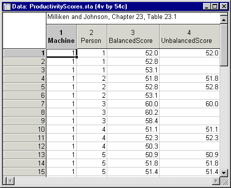
Notice that two dependent variables are reported: BalancedScore and UnbalancedScore. This example will illustrate the ability of Variance Estimation and Precision to analyze balanced models (models where the same number of responses is recorded for each factor combination) and unbalanced models (models where an unequal number of responses is recorded for the factor combinations).

Specifying the Analysis

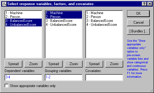
From the Statistics menu, select Variance Estimation and Precision to display the Variance Estimation and Precision Startup Panel, in which you can specify the variables for the design. Click the Variables button, and then select both BalancedScore and UnbalancedScore as Dependent variables. Select Machine and Person as Grouping variables.

Click OK to return to the Startup Panel. Note that STATISTICA automatically selects factor codes; however, if you do not want to use all levels of a particular factor, you can specify the levels you want to use. Simply click the Factor codes button to display the Select codes for indep. vars (factors) dialog and use the options on that dialog to select a subset of factor codes to use in the analysis. Also, you can specify the maximum degree of interactions to include in the default design by entering a value in the Level of interactions field.

For our analysis, we want to use all factor codes and to include the two-way interaction, so click OK on the Startup Panel to display the Define/Review Model dialog. Notice that REML is selected as the default Estimating method, and Type V is selected as the default Sum of squares type. Milliken and Johnson (1992) analyzed these data using the traditional ANOVA approach. To specify this estimation method for both dependent variables, verify that both dependent variables are selected in the Dependents list box (lower right-hand corner) and then select ANOVA in the Estimating method drop-down list.

Dependents

Next we need to specify the sums of squares to use for each dependent variable. You can specify a different estimation method and sum of squares type for each dependent variable by selecting the dependent variable of interest (e.g., BalancedScore) and changing the options on this dialog. For our example, select UnbalancedScore in the Dependents list box, then select the Type I option button in the Sum of squares group box. Next, select BalancedScore in the Dependents list box and the Type III option button in the Sum of squares group box. In the same manner, you can also specify a different custom design for each dependent variable and save those designs to the spreadsheet. We will do this next.

Default designs

When a Variance Estimation and Precision analysis is first launched, STATISTICA generates a default design based on factor coding in the data set. For example, if the indexes of a factor (A) continue to increment across the levels of another factor (B), then in the default design factor A is nested within factor B [A(B)]. This default design is displayed in the Design representation box and is used to generate results in the ANOVA table when no dependent variables have been selected for the analysis. For this spreadsheet, the default design is Machine + Person + Machine*Person indicating that the factor codes suggest a crossed design is appropriate. Note that if you have specified a different design from the one suggested by STATISTICA, you can replace this initial spreadsheet default design with the design specified for the first dependent variable selected in the Dependents list box. To do so, select the Use the design for the first selected dependent variable as the default design to save check box before clicking the Save design button.

Specifying fixed and random effects

Let us continue with our example. Recall that the company in our example was evaluating three brands of machines. Because these three brands of machines are the complete set of possible machines and not a random sample from a larger population of machine brands, Machine is a fixed effect. On the other hand, the six employees who participated in the study are a random sample from the pool of all available employees, and hence, Person is a random effect. To specify fixed and random effects for the BalancedScore model, select BalancedScore in the Dependents list box then click the Customize design button to display the Define Custom Design dialog. In the Effects pane, highlight the effects Person and Machine*Person, and then click the Random button below the pane. Notice that those two effects have changed from fixed to random.

Click OK to return to the Define/Review Model dialog. Notice that the Design representation box has been updated to reflect the current Design effects and Random effects. Next, select UnbalancedScore and specify the same design for that dependent variable.

Saving the designs

Now, let us save this current design by clicking the Save designs button. Once a design has been saved to a spreadsheet, the spreadsheet title bar changes from Data: to Variance Estimation and Precision Designs: indicating that it contains a Variance Estimation and Precision design.

The title bar (see above) also has an asterisk after the spreadsheet name. This indicates that changes have been made to the spreadsheet (i.e., the design metadata was saved to the spreadsheet). If you want to keep the changes you have made to the spreadsheet, you will also need to save it. For spreadsheets with stored Variance Estimation and Precision designs, variable selections are based on the saved design. When the Variance Estimation and Precision module is launched, the first dialog to be displayed will be Define/Review Model dialog.

Reviewing the results

Click OK on the Define/Review Model dialog to display the Variance Estimation and Precision Results dialog. This dialog provides options for reviewing summary results, performing residual analysis, evaluating the variance components (i.e., the contributions to overall variance made by the random effects) and reviewing least squares means for fixed effects. We will begin by reviewing the ANOVA table.

Balanced scores

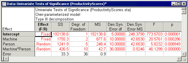
First let us review the results for the BalancedScore response. On the Summary tab, select BalancedScore in the Dependent vars list box (bottom right-hand corner of dialog) then click the ANOVA table button to display the summary ANOVA table for the analysis. This table summarizes the main results of the analysis.

Denominator synthesis

To test the significance of effects in mixed or random models, error terms must be constructed that contain all the same sources of random variation except for the variation of the respective effect of interest. In the Variance Estimation and Precision module when the ANOVA estimation method is used, this is done using Satterthwaite's method of denominator synthesis (Satterthwaite, 1946), which finds the linear combinations of sources of random variation that serve as appropriate error terms for testing the significance of the respective effect of interest. The ANOVA table contains two columns, Den. Syn. Error df and Den. Syn. Error MS, that indicate the appropriate error term to use in tests of significance for each effect and the degrees of freedom associated with that term. Reported F and p values are based on those denominator synthesis mean squares. For example, the F for Machine*Person is the ratio of Machine*Person MS over Error MS (42.6530/.9246) because the two effects have identical sources of variation except for the Machine*Person variation (i.e., the Machine*Person effect has two sources of variation, Machine*Person and Error, while Error only has one source of variation, Error). Within rounding, these estimates agree with those presented by Milliken and Johnson (1992).

Unbalanced scores

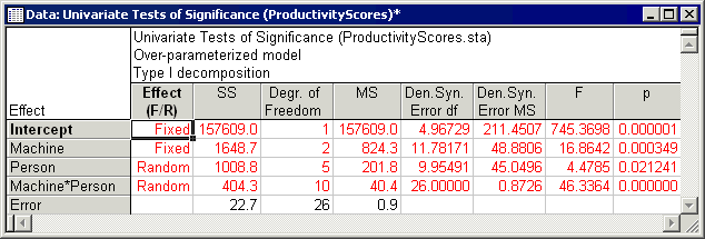
Recall that Milliken and Johnson reported ANOVA results using type I sums of squares for the unbalanced scores. To review similar results in Variance Estimation and Precision, select UnbalancedScore in the Dependent vars list box, then click the ANOVA table button to display the univariate results spreadsheet.

Here again, denominator synthesis error terms have been reported and used. Within rounding, these results also match those reported by Milliken and Johnson.

Variance estimates

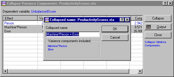
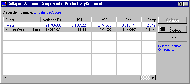
Milliken and Johnson (1992) also reported variance estimates for the UnbalancedScore dependent variable. The Variance Estimation and Precision module provides several ways for reviewing the variance estimates; we will look at two of them. First, click the Collapse variance components button to display the Collapse Variance Components dialog. This dialog shows the variance estimates for each random effect and its degrees of freedom. It also provides an option for collapsing variance components.

As reported in Milliken and Johnson, the variance estimate for Person is 21.7, the variance estimate for Machine*Person is 17.08, and the variance estimate for Error is 0.87. If the Machine*Person variance component was not significant, it might be useful to combine the Machine*Person and Error variance estimates. To do that, select both effects in the Collapse Variance Components dialog, then click the Collapse button. The Collapsed Name dialog will be displayed, enabling you to specify a name for the combined effect.

When you click OK on that dialog, the Collapse Variance Components table will be updated to reflect the combined effect.

Note: you can send the contents of this dialog to a spreadsheet by clicking the Output button. Now, click Close to close this dialog and return to the Summary tab of the Variance Estimation and Precision Results dialog.

You can also review the variance estimates and (if desired) all combined estimates of a specified level using the Collapse table option. First, enter a 2 in the Collapse level edit field to indicate that we want to review all variance component estimates and all possible two-way combined variance estimates. Then click the Collapse table button.

The resulting spreadsheet reports six effects: Person, Machine*Person, Error, Person + Machine*Person, Person + Error, and Machine*Person + Error.

Note: additional options for reviewing and plotting variance estimates are available on the Variance Evaluation tab of the Variance Estimation and Precision Results dialog.

Estimated mean squares

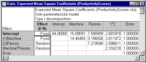
When the ANOVA estimation method has been selected on the Define/Review Model dialog, you can generate a spreadsheet with expected mean square coefficients for each effect. To do this, return to the Summary tab of the Variance Estimation and Precision Results dialog and click the Expected MSs button.

The spreadsheet above shows the coefficients used to construct the linear combinations of sources of variation based on the Type I ANOVA method for the UnbalancedScore dependent variable. The coefficients show, for example, that the Mean square for Machine*Person is calculated as 2.316218 times the variance component for Machine*Person, plus 1.0 times the variance component for Error.