Example 1: Normal Linear Model with Log Link
This example is based on the example data file Income.sta. This data file contains the (fictitious) results of a survey of households in different counties. The data file contains three variables:
Assets: Sum of all assets (in $100,000)
Income: Average taxable income (in $10,000)
County: County where the respective family is located
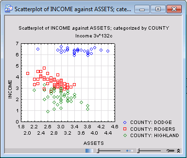
Suppose we are interested in the relationship between Income and Assets within counties, and we want to view a categorized scatterplot.
Open the Income.sta data file and the 2D Categorized Scatterplots Startup Panel. Following are instructions to do this from the ribbon bar and from the classic menus.
Ribbon bar. Select the Home tab. In the File group, click the Open arrow and from the menu, select Open Examples. The Open a STATISTICA Data File dialog box is displayed. Adstudy.sta is located in the Datasets folder.
Then, select the Graphs tab. In the More group, click the Categorized arrow and select Scatterplots to display the 2D Categorized Scatterplots Startup Panel.
Classic menus. From the File menu, select Open Examples to display the Open a STATISTICA Data File dialog box; Income.sta is located in the Datasets folder.
Then, select Scatterplots from the Graphs - Categorized Graphs submenu to display the 2D Categorized Scatterplots Startup Panel.

On the Quick tab in the Layout group box, select the option button.
Click the Variables button to display the standard variable selection dialog box. Select Assets as the X variable, Income as the Y variable, County as the X-Category variable, and then click the OK button.
Finally, click the OK button in the 2D Categorized Scatterplots Startup Panel. The following categorized scatterplot of Income and Assets by County may suggest a normal linear model with log link and separate slopes.
Specifying the Analysis
- Open the
Generalized Linear/Nonlinear Models module in the following ways:
- Ribbon bar. Select the Statistics tab. In the Advanced/Multivariate group, click Advanced Models and select Generalized Linear/Nonlinear to display the Generalized Linear/Nonlinear Models Startup Panel.
- Classic menus. Select Generalized Linear/Nonlinear Models from the Statistics - Advanced Linear/Nonlinear Models submenu to display the Generalized Linear/Nonlinear Models Startup Panel.
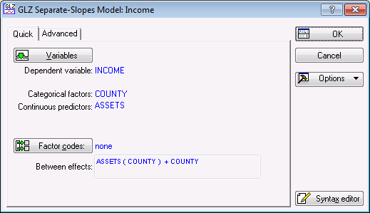
- On the Advanced tab in the Type of analysis group box, select Separate-slopes model.
- In the Specification method group box, select Quick specs dialog box.
- In the Distribution group box, select Normal.
- In the Link functions group box, select Log.
- Then, click the OK button to display the GLZ Separate-Slopes Model Quick Specs dialog box.
- Click the Variables button to display the standard variable selection dialog box.
- Select Income as the Dependent (response) variable, County as the Categ. (factors), Assets as the Continuous predictors variable (covariate), and then click the OK button. The GLZ Separate-Slopes Model Quick Specs dialog box is displayed.
- Click the OK button to display the GLZ Results dialog box. During the estimation procedure, you see a warning message informing you that one of the parameters in the model was set to zero; the reason for this is that for the Separate-slopes model, Statistica uses the overparameterized parameterization of the categorical predictor County; in order to estimate a solution (parameter estimates) for this mode, one of the parameters must be set to zero (for details, see also the Introductory Overview section of the GLM module). Simply click the OK button in the warning message dialog box.
- If you want to run this example using GLZ Syntax, you can run the following syntax program from the GLZ Analysis Syntax Editor dialog box (see Methods for Specifying Designs).
Parameter Estimates
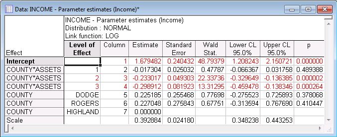
The spreadsheet shows the parameter estimates for each column in the design matrix. It appears that two of the three parameters for the County by Assets interaction (the separate slopes) are statistically significant.
Goodness of Fit
Next, let us see whether, overall, this model provides a good fit to the data. Click the Goodness of fit button, under Sample, to display the Statistics of goodness of fit spreadsheet.

It appears that the Separate-slopes model reproduces the data well.
Model Checking - Heterogeneous variances
Next, select the Resid. 1 tab, and click the Pred. & resids button under Plots of predicted and residual values to produce a scatterplot of the residual and predicted values.
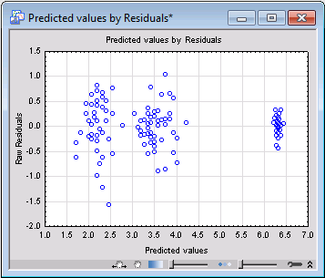
Apparently, the variance of the residuals is not homogeneous over the groups (counties) in the model. Thus, you can fit completely separate regression models for each county.
Outlier Detection

In this example, the 71st data point (you can use the Brushing tools to label the outlier shown on the right side of the graph) has a large Chi-square value, and thus is the largest contributor to the lack of fit for this model.