Example 1: Predicting Success/Failure
- Overview
- The examples for Nonlinear Estimation are mostly based on demonstration data sets provided in Neter, Wasserman, and Kutner (1985). The discussion of these examples will focus primarily on how to specify models and how to interpret results. Additional guidelines for cases when the estimation procedure fails or for dealing with unusual cases are also provided.
The logit and probit models for binary dependent variables will first be reviewed; these models are "pre-wired" into the Nonlinear Estimation module and can be chosen as dialog options. Numerous examples of how to fit models and use different loss functions specified by the user will then be reviewed. Note that Logistic (Logit) and Probit regression models can also be fit using the Generalized Linear/Nonlinear Models (GLZ) facilities of STATISTICA; GLZ contains options for fitting ANOVA and ANCOVA-like designs to binomial and multinomial response variables, and provides methods for stepwise and best-subset selection of predictors.
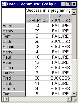
This example is based on a data set described in Neter, Wasserman, and Kutner (1985, page 357; however, note that those authors fit a linear regression model to the data). Suppose you want to study whether experience helps programmers complete complex programming tasks within a specified amount of time. Twenty-five programmers were selected with different degrees of experience (measured in months). They were then asked to complete a complex programming task within a certain amount of time. The binary dependent variable is the programmers' success or failure in completing the task. These data are recorded in the file Program.sta; shown below is a partial listing of this file.
- Specifying the analysis
- After starting STATISTICA, open the Program.sta data file by selecting Open Examples from the File menu (classic toolbar) or by selecting Open Examples from the Open menu on the Home tab (ribbon bar); it is in the Datasets folder. Then select Nonlinear Estimation from the Statistics - Advanced Linear/Nonlinear Models submenu to display the Nonlinear Estimation Startup Panel.
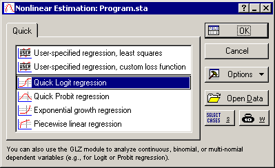
Double-click Quick Logit regression on the Quick tab to display the Logistic Regression (Logit) dialog.
Next, click the Variables button to display the standard variable selection dialog and select the variable Success from the Dichotomous dependent variable list and Expernce from the Continuous independent variable list. Click the OK button.
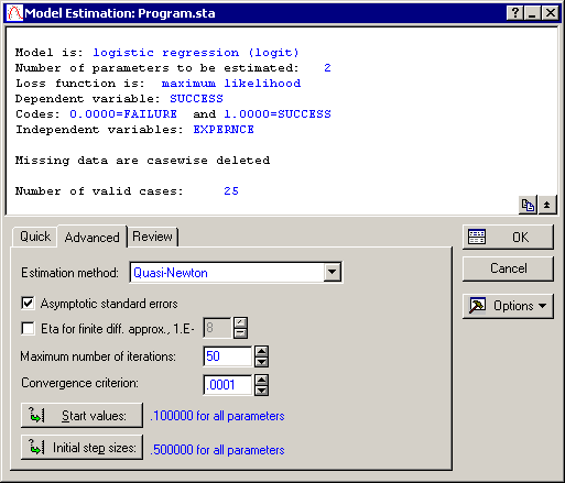
STATISTICA will automatically enter the codes for the dependent variable in this dialog. You can also specify the type of missing data deletion (Casewise deletion of missing data or Mean substitution of missing data).
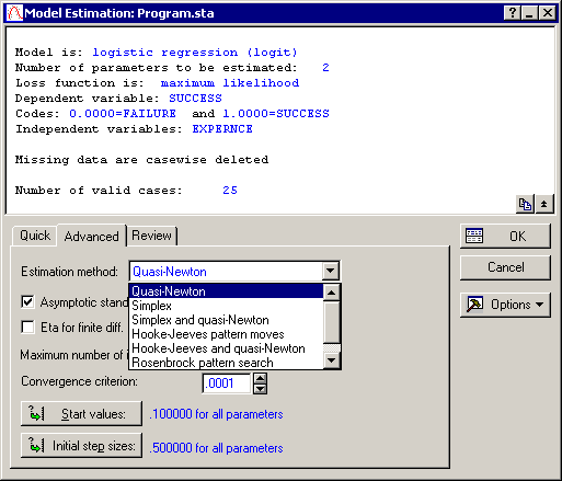
Note: the Nonlinear Estimation module will always compute maximum likelihood parameter estimates for logit and probit models. Ordinary least squares estimation is based on the assumption of constant error (or residual) variance at different values of the independent variables. In the case of binary dependent variables, this assumption is clearly violated, and thus, the maximum likelihood criterion should be used to estimate the parameters of the logistic (and probit) regression model.Accept the program defaults and click the OK button in the Logistic Regression (Logit) dialog to display the Model Estimation dialog. In this dialog, you can select the estimation method as well as specify the convergence criterion, start values, etc. You can also elect to compute separately (via finite difference approximation) the asymptotic standard errors for the parameter estimates. For this example, on the Advanced tab, select the Asymptotic standard errors check box .
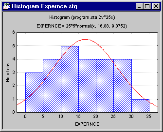
To review the descriptive statistics for all selected variables, on the Review tab, click the Means & standard deviations button. As in most other descriptive statistics spreadsheets in STATISTICA, the default graph is the histogram with the normal curve superimposed (right-click on the EXPERNCE column in the spreadsheet and select Graphs of Input Data - Histogram EXPERNCE - Normal Fit from the resulting shortcut menu). Thus, you could at this point evaluate the distributions of the variables.
The different estimation procedures in the Nonlinear Estimation module are discussed in the Introductory Overviews. Click the Estimation method drop-down box on the Advanced tab of the Model Estimation dialog to see the different options.
A good way to start the analysis is with the default settings in this dialog. As discussed in the Introductory Overviews, all estimation procedures require as input start values, initial step sizes, and the convergence criterion. Again, simply accept the defaults as shown in this dialog and click the OK button to estimate the parameters.
- Estimating the parameters
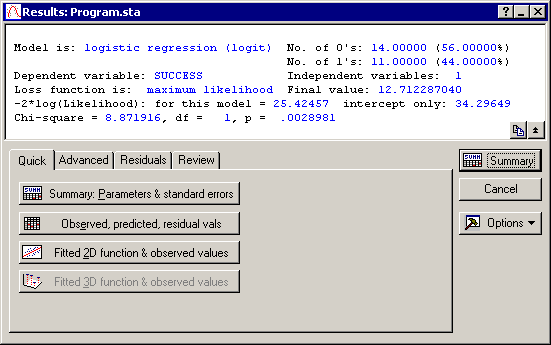
- STATISTICA briefly displays in a window the values of the loss function and the current estimate for each parameter at each iteration. After a few iterations the Quasi-Newton estimation procedure will converge, that is, arrive at the final parameter estimates and the Results dialog is displayed.
- Reviewing results
- The Chi-square value for the difference between the current model and the intercept-only model is highly significant (.003). Thus, one can conclude that experience is related to programmers' success.
Now, review the parameter estimates by clicking the Summary: Parameters & standard errors button on the Results dialog - Quick tab. As described in the Introductory Overviews, the standard errors are computed from the finite difference approximation of the Hessian matrix of second-order derivatives. By dividing the estimates by their respective standard errors, you can compute approximate t-values, and thus compute the statistical significance levels for each parameter. The results in the spreadsheet show that both parameters are significant at the p<.05 level.
- Estimation of standard errors
- The Model: Logistic regression (logit) results spreadsheet shows that the loss was calculated using Maximum Likelihood with MS-err. scaled to 1. In fact, in maximum likelihood estimation, it is a common practice to rescale the mean square error to 1.0 when computing the estimates for the parameter standard errors (see Jennrich and Moore, 1975, for details).
- Interpreting the parameter estimates
- In principle, the parameter estimates can be interpreted as in standard linear regression, that is, in terms of an intercept (Const.B0) and slope (Expernce). Thus, essentially, the results of this study show that the amount of prior experience is significantly related to the successful completion of the programming task. However, as described in the Introductory Overviews, the parameter estimates pertain to the prediction of logits (computed as log[p/(1-p)]), not the actual probabilities (p) underlying success or failure. Logits will assume values from minus infinity to plus infinity, as the probability p moves from 0 to 1.
- Predicted values
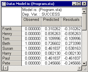
- Now examine the predicted values. Click the Observed, predicted, residual vals button on the
Results - Residuals tab to view the predicted values of the dependent variable Success (second column in the results spreadsheet). Remember that the logit regression model ensures that the predicted values will never step out of the 0-1 bounds. Thus, you may look at the predicted values as probabilities; for example, the predicted probability of success for the second case (Henry) is (.84).
Note: you can also save the predicted and residual values for further analysis via the Save predicted and residual values button on the Residuals tab.
- Classification of cases
- Click the Classification of cases & odds ratio button on the
Residuals tab to display the table of correctly and incorrectly classified cases, given the current model (i.e., the current parameter estimates).
All cases with a predicted value (probability) less than or equal to .5 are classified as Failure, those with a predicted value greater than .5 are classified as Success. The Odds ratio is computed as the ratio of the product of the correctly classified cases over the product of the incorrectly classified cases. Odds ratios that are greater than 1 indicate that the classification is better than what one would expect by pure chance. However, remember that these are post-hoc classifications, because the parameters were computed so as to maximize the probability of the observed data (see the description of the maximum likelihood loss function in the Introductory Overviews). Thus, you should not expect to do this well if you applied the current model to classify new (future) observations.
- Normal probability plot
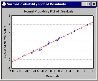
- The Introductory Overviews discuss how normal and half-normal probability plots are constructed. Now click the Normal probability plot of residuals button on the
Residuals tab to produce this graph.
If the residuals (observed minus predicted values) are normally distributed, they will fall approximately onto a straight line in the normal probability plot. In the current example, essentially all points (residuals) in the normal probability plot are very close to the line, indicating that the residuals are normally distributed.
- Histogram of residuals
- Another quick visual way to inspect the distribution of the residuals is through the histogram. Click the Histogram of residuals button on the
Residuals tab to create the Frequency Distribution: Residuals plot.
Again, it appears from this plot that the residuals are basically normally distributed.
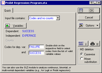
- Fitting a probit model
- For comparison, now fit the probit regression model to these data. Click the Cancel button in the
Results dialog and again in the
Logistic Regression (Logit) dialog to return to the Nonlinear Estimation Startup Panel. Double-click Quick Probit regression on the Quick tab. In the
Probit Regression dialog, click the Variables button, and select Success in the Dichotomous dependent variable list and Expernce in the Continuous independent variable list; then click the OK button.
Click the OK button in the Probit Regression dialog to display the Model Estimation dialog.
Now, click the OK button to display the Results dialog.
- Reviewing results
- As before, the Chi-square value (0.003) for the comparison of the current model with the intercept-only model is statistically significant. In fact, the Chi-square value is practically the same as before. Thus, the probit regression also leads to the conclusion that programming experience is significantly related to success.
- Interpreting the parameter estimates
- The parameter estimates for the probit regression can also be interpreted as in standard linear regression. However, the parameter estimates in probit regression pertain to the prediction of z values of the normal distribution. If you then take the normal integral of those z values, you end up with values that will never step out of the 0-1 boundaries. The predicted values can again be thought of as probabilities, in this case, as the space under the normal curve associated with the respective predicted z value.
Now, on the Results dialog - Residuals tab, click the Observed, predicted, residual vals button to look at the predicted values of the dependent variable Success.
As you can see in the results spreadsheet above, the predicted values (probabilities of success) for each case under the probit model are very similar to those for the logit model. In fact, in most cases, the difference between these two models is negligible.
- Incremental fit with more than one variable
- Before concluding this example, there is an additional feature when fitting probit or logit models that will be discussed. If there are, for example, two independent variables, you can first estimate the model with one variable, and then the model with both variables. In this case, the Difference from previous model button on the Results dialog - Advanced tab will no longer be dimmed. This option will compute the difference in the loss function (maximum likelihood) from the previous model (with one independent variable) to the current model (with two independent variables). The Chi-square value and p-value for the increment in goodness of fit is also reported. In general, you can enter or remove in successive analyses one or more variables; if the resulting model is a subset or superset of the previously fitted model, the incremental goodness of fit will automatically be computed.