Box-Cox Transformation Overview and Technical Notes
Often it is important to transform the variables of a data set in a suitable way before performing any analysis or modeling. This procedure, that is, the transformation of the raw (original) data in a way that will aid the subsequent modeling and analysis, is generally known as pre-processing. For example, suppose that we have a data set consisting of two variables, an independent (predictor) variable X and a dependent (predicted) variable Y. When performing a fit of Y against X often an appropriate transformation of the variables may significantly improve the quality of the fit.
Such techniques have proven to be very useful in a variety of statistical modeling including regression analysis. More generally, many statistical analyses only work under the normality condition and, therefore, transforming the original variable to a normal distribution allows the application of many statistical techniques that otherwise are invalid should the normality assumption not hold sufficiently well.
One particular family of such transformations that aims at transforming the original data in a way that the new variable has a distribution as close to normality as possible is known as the Box-Cox method (Box and Cox, 1964). With
![]() being the transformation parameter, the Box-Cox formula can be written as,
being the transformation parameter, the Box-Cox formula can be written as,
where
![]() is the variable being transformed, and
is the variable being transformed, and
![]() is known as the shift parameter.
is known as the shift parameter.
The aim of the Box-Cox transformation is to convert the variable X in a way that the resulting new variable
![]() has a distribution as close as it can to normality, that is,
has a distribution as close as it can to normality, that is,
![]() with mean
with mean
![]() and standard deviation
and standard deviation
![]() ,
,
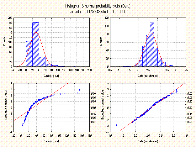
The preceding figure illustrates the effect of the Box-Cox transformation on a variable (data) that has a non-normal distribution (left side figures). After applying the transformation the new variable (transformed) has a distribution that is substantially closer to normality (right side figures) as compared to its distribution prior to the transformation.
To apply the Box-Cox transformation, we need to find a suitable value of
![]() , denoted by
, denoted by
![]() , that yields a transformed variable with a distribution close to normality. There are several techniques to approach this problem, that is, to find the optimal value of
, that yields a transformed variable with a distribution close to normality. There are several techniques to approach this problem, that is, to find the optimal value of
![]() that satisfies the normality assumption best. The approach used by
Statistica is known as the
maximum likelihood approach, in which we construct a likelihood function (or rather an error criterion E defined as minus logarithm of the likelihood function),
that satisfies the normality assumption best. The approach used by
Statistica is known as the
maximum likelihood approach, in which we construct a likelihood function (or rather an error criterion E defined as minus logarithm of the likelihood function),
where
![]() is the standard deviation of the transformed variable
is the standard deviation of the transformed variable
![]() . The value of
. The value of
![]() , which minimizes the above equation, is our optimal
, which minimizes the above equation, is our optimal
![]() for the Box-Cox transformation.
for the Box-Cox transformation.
Finding
![]() requires an iterative procedure. Statistica Box-Cox uses the so called Golden Search. In this algorithm we start with a minimum value of lambda, apply the Box-Cox transformation and calculate the error function above. This process is repeated over and over again for various values of lambda (not exceeding a given maximum range) until a suitable lambda is found for which the error function is minimum.
requires an iterative procedure. Statistica Box-Cox uses the so called Golden Search. In this algorithm we start with a minimum value of lambda, apply the Box-Cox transformation and calculate the error function above. This process is repeated over and over again for various values of lambda (not exceeding a given maximum range) until a suitable lambda is found for which the error function is minimum.
See also, Box-Cox Transformation and Box-Cox Transformation Results.


