Example 4: Estimating the Population Intraclass Correlation in Variance Estimation and Precision
- Specifying the Design
- This example illustrates how to estimate the population intraclass correlation coefficient for a random factor using variance component estimation (Hays, 1988, pp. 483-490). The value of the population intraclass correlation coefficient is a measure of the homogeneity of observations within the classes of a random factor relative to the variability of such observations between classes. It will be zero when the estimated effect of the random factor is zero and will reach unity only when the estimated effect of error is zero, given that the total variation of the observations is greater than zero (see Hays, 1988, p. 485).
Example 4 is based on an example data set presented by Hays (1988, p. 484). Five different experimenters chosen at random each administered 2 tests to 8 subjects. The independent variable is Tester and the dependent variables are Y1 and Y2. Y1 is the same dependent variable presented in the example by Hays (1988, p. 484). There are significant differences in the means on Y1 for different Testers (see Table 13.4.2 in Hays, 1988, p. 484). Y2 is a transformation of Y1 such that it has the same within-Tester variation as Y1, but identical means for each Tester. The data are available in the example data file Hays484.sta (a partial listing of this data file is shown below). Open this data file via the File - Open Examples menu; it is in the Datasets folder.
To perform the analysis, select Variance Estimation and Precision from the Statistics menu to display the Variance Estimation and Precision Startup Panel.
On the Quick tab, click the Variables button to display the standard variable selection dialog. Here, clear the Show appropriate variables only checkbox. Then select variable Y1 and Y2 as the Dependent variables, variable Tester as the Grouping variable and then click the OK button to display the Define/Review Model dialog.
For this example we will estimate variance components using the ANOVA-based Type I expected mean squares method. Select ANOVA in the Estimating method drop-down list, then select the Type I option button in the Sums of squares group box.
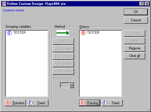
Next, click the Customize design button to display the Define Custom Design dialog. In the Effects pane, select Tester, then click the Random button.
Click OK on this dialog to return to the Define/Review Model dialog, then click OK to display the Variance Estimation and Precision Results dialog. On the Variance evaluation tab, select Y1 in the Dependent vars list box and click the Variance estimates button to display the Components of Variance spreadsheet for Y1.
The population intraclass correlation coefficient for Tester on Y1 is computed as the ratio of the estimated variance component for Tester on Y1 to the sum of the Tester and Error variance components on Y1. For this example the population intraclass correlation coefficient for Tester on Y1 is computed as .098645 / (.179859), or .55, indicating that 55% (as shown in the Percent column) of the variation on Y1 is accounted for by Tester.
Return to the Variance evaluation tab of the Variance Estimation and Precision Results dialog, and select Y2 in the Dependent vars list box. Again, click the Variance estimates button to display the Components of Variance spreadsheet for Y2.
The results for the population intraclass correlation coefficient for Tester on Y2 are quite different. Notice that the variance estimate for Tester is shown in orange, indicating that the original variance estimate was negative. A negative variance estimate cannot logically be taken as indicating that a negative percentage of the variation on Y2 is accounted for by Tester, because variation, by definition, is positive. It is instead taken as indicating that the variance component for Tester is zero, that the population intraclass correlation coefficient for Tester on Y2 is zero, and that 0% of the variation on Y2 is accounted for by Tester. A seemingly negative variance component for Tester on Y2 can easily be understood by comparing the Mean squares for Tester and for Error from the ANOVA. To display the Univariate Tests of Significance spreadsheet for Y1 and Y2, select both variables in the Dependent vars box, then click the ANOVA button. Two spreadsheets will be displayed.
Y2 has exactly the same within Tester class variation as Y1, but no differences in Tester class means. Thus the Mean square for Tester on Y2 is zero, which is less than the Mean square for Error. The negative variance component estimate for Tester on Y2 simply reflects the fact that observations are less homogeneous (i.e., have more variation) within classes of Tester than between classes of Tester.
Note: estimated intraclass correlation coefficients are displayed on stacked bar plots and pie charts when the Plot relative variances (% of total) check box is selected (see the Variance Estimation and Precision Results - Variance Evaluation tab). Shown below is the compound graph that is produced when you click the Stacked bar for var. estimates button.These relative variances can be interpreted as zero-order intraclass correlations when there is only one random factor in the analysis. If there is more than one random effect in the analysis and the random effects are correlated, the relative variances should be interpreted as partial intraclass correlations.
See Variance Estimation and Precision Index.