Example 3: Discriminant-Based Linear Combination Splits for Ordered Predictors
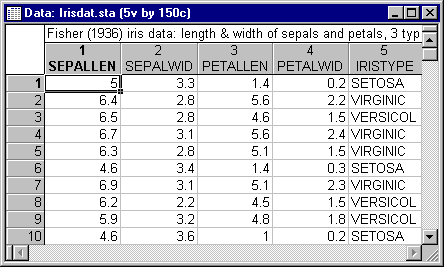
This example is based on a classic example data set reported by Fisher (1936). This same data set is used to illustrate linear discriminant analysis in the Discriminant Analysis module. The data file for this analysis is Irisdat.sta. Open this data file via the File - Open Examples menu; it is in the Datasets folder. A partial listing of this file is shown below. The first two variables in this file (Sepallen, Sepalwid), pertain to the length and width of sepals; the next two variables (Petallen, Petalwid) pertain to the length and width of petals. The last variable (Iristype) contains code for the observed classifications of each flower as Setosa, Versicol, or Virginica. In all, there are 150 flowers in this sample, 50 of each type.
Specifying the analysis
This example uses the program defaults for all options except for the specification of Discriminant-based linear combination splits for ordered predictors as the Split selection method. Select Classification Trees from the Statistics - Multivariate Exploratory Techniques menu to display the Classification Trees Startup Panel. On the Quick tab, select the Variables button to display the standard variable selection dialog. Here, select Iristype as the Dependent variable, the four measurement variables as the Ordered predictors, and then click the OK button. On the Methods tab, select the Discriminant-based linear combination splits for ordered predictors under Split selection method. Finally, click the OK button on the Classification Trees Startup Panel to first briefly display the Parameter Estimation dialog (from which you can monitor the progress of the classification tree computations) and then the Classification Trees Results dialog when the computations are completed.
Reviewing the results
On the Tree structure tab, click the Split conditions button to display a spreadsheet showing the coefficients for the linear combination splits for the selected classification tree.
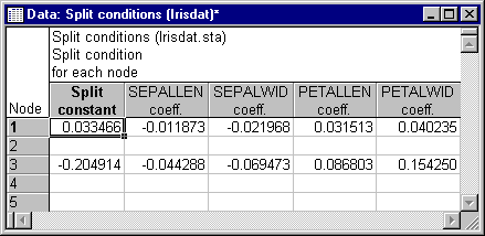
The spreadsheet shows that the selected tree has two splits, which occur at Node 1 and Node 3. The Node 1 split, for example, specifies that cases for which the function .033466 + (-.011873 * SEPALLEN) + ( -.021968 * SEPALWID) + (.031513 * PETALLEN) + (.040235 * PETALWID) has a value of less than or equal to zero would be sent to the left child node of Node 1. All other cases would be sent to the right child node of Node 1. Now click the Misclassification matrix button on the Predicted classes tab to display the spreadsheet shown below.
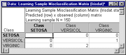
This spreadsheet shows that for the selected tree 3 out of the 150 flowers, or 2% were misclassified.
It is coincidental that the selected classification tree has two linear combination splits, the same as the number of linear discriminant functions that can be extracted (the number of linear discriminant functions that can be extracted is the lesser of the number of predictors or the number of classes on the dependent variable minus 1, i.e., 2 for this data set). Linear combination splits for classification trees do not have a restriction on the number of splits as does linear discriminant analysis. To illustrate this, return to the Classification Trees Startup Panel (by clicking the Cancel button) and select the FACT-style direct stopping option button under Stopping rule on the Stopping options tab. Enter .02 in the Fraction of objects field (which corresponds to a minimum class size of 1 for terminal nodes, since there are 50 cases in each class and 50 times .02 equals one). Now, click the OK button to display the Classification Trees Results dialog. Then generate the Split conditions and Learning Sample Misclassification Matrix spreadsheets as described above. You will see that in the analysis there are 9 linear combination splits that produce perfect prediction of Iristype. It has taken 7 additional linear combination splits to accurately predict the 2% of cases misclassified in the first analysis.
See also Classification Trees Index.